Crypto Candlestick Patterns - CN VersionIntroduction:
The candlestick chart has been used for centuries since the Japanese applications. Based on the candlestick charting, people developed candle pattern analysis. Now we have tons of books or articles illustrating the usage of reversal patterns and continuation patterns, and computers provide a faster and preciser way to recognize these pattern.
Originally we have a common *All Candlestick Patterns* indicator to use. This indicator works well for most of the markets or commodities including stocks and futures. However, for cryptocurrency market, quite a few patterns are not suitable anymore. For example, crypto markets are continuously running 7x24hrs and the big coins with good volume tend to have almost continuous price in commonly used time periods. Hence, original patterns with "window" or "jump" concepts are usually not applied to crypto.
For these issues, I modified the original *All Candlestick Patterns* indicator and introduced the Chinese version for people speaking such language.
Like most of the other indicators, I personally do not recommend anyone to simply follow the patterns it shows to enter the market. You may take these recognized patterns as a reference, and further actions on trading should be done with several other tools, such as MACD, RSI, Stochastic and etc.
Usage:
The application of this indicator is basically the same as the original *All Candlestick Patterns* and you will get an automatically generated pattern recognition by your computer system.
There are a few parameters to adjust for the indicator:
Trending Detection Settings: Here you can choose SMA-Fast, SMA-Fast/Slow or None detecting options to recognize the current market trend. This is a minor improvement from the original indicator and you can choose your preferred trending detecting settings by changing the length of SMA.
Candlestick Settings: You may adjust the rules to recognize the properties of candlesticks. I add a "perturbation" parameter here, which actually is an error tolerance for pattern recognition. Some seemingly pattern may not fulfill the strict rules of classic candlestick patterns, but we may recognize them by watch the charting on our own. Hence this error tolerance may show more potential patterns from the charting.
Plot Settings: It is the usually colour choice and providing options for bullish/bearish.
Pattern Settings: Here you can select the patterns that you would like to see from the charting. You can pick the preferred reversal patterns or choose to show all the patterns. It's all up to you!
Features:
Language Translation: Since this is a Chinese language version. I have replaced all the English explanation of patterns to Chinese ones. Move your mouse to the label, you will find a brief intro of the pattern and a notice about bullish or bearish signals it indicates.
Alerts: As the same as the original one, we will have the alert options from this indicator. All the alerts and their messages are Chinese. You can activate alerts based on this indicator from the alert management section, as the same as many other indicators you have used before.
Future Improvements:
For now I am satisfied with the work I have done, and I may apply it to several charts. It's welcome for any users to take a look at the codes and put modifications or improvements towards it. Currently most of the comments in the code are in Chinese language, since basically it's for Chinese speaking users, while the code itself and the parameter names should be pretty easy to understand in English. (I have been using English for writing in the past 8 years, hence this introduction is in English as well.)
Search in scripts for "Pattern recognition"

Quantum Rotational Field MappingQuantum Rotational Field Mapping (QRFM):
Phase Coherence Detection Through Complex-Plane Oscillator Analysis
Quantum Rotational Field Mapping applies complex-plane mathematics and phase-space analysis to oscillator ensembles, identifying high-probability trend ignition points by measuring when multiple independent oscillators achieve phase coherence. Unlike traditional multi-oscillator approaches that simply stack indicators or use boolean AND/OR logic, this system converts each oscillator into a rotating phasor (vector) in the complex plane and calculates the Coherence Index (CI) —a mathematical measure of how tightly aligned the ensemble has become—then generates signals only when alignment, phase direction, and pairwise entanglement all converge.
The indicator combines three mathematical frameworks: phasor representation using analytic signal theory to extract phase and amplitude from each oscillator, coherence measurement using vector summation in the complex plane to quantify group alignment, and entanglement analysis that calculates pairwise phase agreement across all oscillator combinations. This creates a multi-dimensional confirmation system that distinguishes between random oscillator noise and genuine regime transitions.
What Makes This Original
Complex-Plane Phasor Framework
This indicator implements classical signal processing mathematics adapted for market oscillators. Each oscillator—whether RSI, MACD, Stochastic, CCI, Williams %R, MFI, ROC, or TSI—is first normalized to a common scale, then converted into a complex-plane representation using an in-phase (I) and quadrature (Q) component. The in-phase component is the oscillator value itself, while the quadrature component is calculated as the first difference (derivative proxy), creating a velocity-aware representation.
From these components, the system extracts:
Phase (φ) : Calculated as φ = atan2(Q, I), representing the oscillator's position in its cycle (mapped to -180° to +180°)
Amplitude (A) : Calculated as A = √(I² + Q²), representing the oscillator's strength or conviction
This mathematical approach is fundamentally different from simply reading oscillator values. A phasor captures both where an oscillator is in its cycle (phase angle) and how strongly it's expressing that position (amplitude). Two oscillators can have the same value but be in opposite phases of their cycles—traditional analysis would see them as identical, while QRFM sees them as 180° out of phase (contradictory).
Coherence Index Calculation
The core innovation is the Coherence Index (CI) , borrowed from physics and signal processing. When you have N oscillators, each with phase φₙ, you can represent each as a unit vector in the complex plane: e^(iφₙ) = cos(φₙ) + i·sin(φₙ).
The CI measures what happens when you sum all these vectors:
Resultant Vector : R = Σ e^(iφₙ) = Σ cos(φₙ) + i·Σ sin(φₙ)
Coherence Index : CI = |R| / N
Where |R| is the magnitude of the resultant vector and N is the number of active oscillators.
The CI ranges from 0 to 1:
CI = 1.0 : Perfect coherence—all oscillators have identical phase angles, vectors point in the same direction, creating maximum constructive interference
CI = 0.0 : Complete decoherence—oscillators are randomly distributed around the circle, vectors cancel out through destructive interference
0 < CI < 1 : Partial alignment—some clustering with some scatter
This is not a simple average or correlation. The CI captures phase synchronization across the entire ensemble simultaneously. When oscillators phase-lock (align their cycles), the CI spikes regardless of their individual values. This makes it sensitive to regime transitions that traditional indicators miss.
Dominant Phase and Direction Detection
Beyond measuring alignment strength, the system calculates the dominant phase of the ensemble—the direction the resultant vector points:
Dominant Phase : φ_dom = atan2(Σ sin(φₙ), Σ cos(φₙ))
This gives the "average direction" of all oscillator phases, mapped to -180° to +180°:
+90° to -90° (right half-plane): Bullish phase dominance
+90° to +180° or -90° to -180° (left half-plane): Bearish phase dominance
The combination of CI magnitude (coherence strength) and dominant phase angle (directional bias) creates a two-dimensional signal space. High CI alone is insufficient—you need high CI plus dominant phase pointing in a tradeable direction. This dual requirement is what separates QRFM from simple oscillator averaging.
Entanglement Matrix and Pairwise Coherence
While the CI measures global alignment, the entanglement matrix measures local pairwise relationships. For every pair of oscillators (i, j), the system calculates:
E(i,j) = |cos(φᵢ - φⱼ)|
This represents the phase agreement between oscillators i and j:
E = 1.0 : Oscillators are in-phase (0° or 360° apart)
E = 0.0 : Oscillators are in quadrature (90° apart, orthogonal)
E between 0 and 1 : Varying degrees of alignment
The system counts how many oscillator pairs exceed a user-defined entanglement threshold (e.g., 0.7). This entangled pairs count serves as a confirmation filter: signals require not just high global CI, but also a minimum number of strong pairwise agreements. This prevents false ignitions where CI is high but driven by only two oscillators while the rest remain scattered.
The entanglement matrix creates an N×N symmetric matrix that can be visualized as a web—when many cells are bright (high E values), the ensemble is highly interconnected. When cells are dark, oscillators are moving independently.
Phase-Lock Tolerance Mechanism
A complementary confirmation layer is the phase-lock detector . This calculates the maximum phase spread across all oscillators:
For all pairs (i,j), compute angular distance: Δφ = |φᵢ - φⱼ|, wrapping at 180°
Max Spread = maximum Δφ across all pairs
If max spread < user threshold (e.g., 35°), the ensemble is considered phase-locked —all oscillators are within a narrow angular band.
This differs from entanglement: entanglement measures pairwise cosine similarity (magnitude of alignment), while phase-lock measures maximum angular deviation (tightness of clustering). Both must be satisfied for the highest-conviction signals.
Multi-Layer Visual Architecture
QRFM includes six visual components that represent the same underlying mathematics from different perspectives:
Circular Orbit Plot : A polar coordinate grid showing each oscillator as a vector from origin to perimeter. Angle = phase, radius = amplitude. This is a real-time snapshot of the complex plane. When vectors converge (point in similar directions), coherence is high. When scattered randomly, coherence is low. Users can see phase alignment forming before CI numerically confirms it.
Phase-Time Heat Map : A 2D matrix with rows = oscillators and columns = time bins. Each cell is colored by the oscillator's phase at that time (using a gradient where color hue maps to angle). Horizontal color bands indicate sustained phase alignment over time. Vertical color bands show moments when all oscillators shared the same phase (ignition points). This provides historical pattern recognition.
Entanglement Web Matrix : An N×N grid showing E(i,j) for all pairs. Cells are colored by entanglement strength—bright yellow/gold for high E, dark gray for low E. This reveals which oscillators are driving coherence and which are lagging. For example, if RSI and MACD show high E but Stochastic shows low E with everything, Stochastic is the outlier.
Quantum Field Cloud : A background color overlay on the price chart. Color (green = bullish, red = bearish) is determined by dominant phase. Opacity is determined by CI—high CI creates dense, opaque cloud; low CI creates faint, nearly invisible cloud. This gives an atmospheric "feel" for regime strength without looking at numbers.
Phase Spiral : A smoothed plot of dominant phase over recent history, displayed as a curve that wraps around price. When the spiral is tight and rotating steadily, the ensemble is in coherent rotation (trending). When the spiral is loose or erratic, coherence is breaking down.
Dashboard : A table showing real-time metrics: CI (as percentage), dominant phase (in degrees with directional arrow), field strength (CI × average amplitude), entangled pairs count, phase-lock status (locked/unlocked), quantum state classification ("Ignition", "Coherent", "Collapse", "Chaos"), and collapse risk (recent CI change normalized to 0-100%).
Each component is independently toggleable, allowing users to customize their workspace. The orbit plot is the most essential—it provides intuitive, visual feedback on phase alignment that no numerical dashboard can match.
Core Components and How They Work Together
1. Oscillator Normalization Engine
The foundation is creating a common measurement scale. QRFM supports eight oscillators:
RSI : Normalized from to using overbought/oversold levels (70, 30) as anchors
MACD Histogram : Normalized by dividing by rolling standard deviation, then clamped to
Stochastic %K : Normalized from using (80, 20) anchors
CCI : Divided by 200 (typical extreme level), clamped to
Williams %R : Normalized from using (-20, -80) anchors
MFI : Normalized from using (80, 20) anchors
ROC : Divided by 10, clamped to
TSI : Divided by 50, clamped to
Each oscillator can be individually enabled/disabled. Only active oscillators contribute to phase calculations. The normalization removes scale differences—a reading of +0.8 means "strongly bullish" regardless of whether it came from RSI or TSI.
2. Analytic Signal Construction
For each active oscillator at each bar, the system constructs the analytic signal:
In-Phase (I) : The normalized oscillator value itself
Quadrature (Q) : The bar-to-bar change in the normalized value (first derivative approximation)
This creates a 2D representation: (I, Q). The phase is extracted as:
φ = atan2(Q, I) × (180 / π)
This maps the oscillator to a point on the unit circle. An oscillator at the same value but rising (positive Q) will have a different phase than one that is falling (negative Q). This velocity-awareness is critical—it distinguishes between "at resistance and stalling" versus "at resistance and breaking through."
The amplitude is extracted as:
A = √(I² + Q²)
This represents the distance from origin in the (I, Q) plane. High amplitude means the oscillator is far from neutral (strong conviction). Low amplitude means it's near zero (weak/transitional state).
3. Coherence Calculation Pipeline
For each bar (or every Nth bar if phase sample rate > 1 for performance):
Step 1 : Extract phase φₙ for each of the N active oscillators
Step 2 : Compute complex exponentials: Zₙ = e^(i·φₙ·π/180) = cos(φₙ·π/180) + i·sin(φₙ·π/180)
Step 3 : Sum the complex exponentials: R = Σ Zₙ = (Σ cos φₙ) + i·(Σ sin φₙ)
Step 4 : Calculate magnitude: |R| = √
Step 5 : Normalize by count: CI_raw = |R| / N
Step 6 : Smooth the CI: CI = SMA(CI_raw, smoothing_window)
The smoothing step (default 2 bars) removes single-bar noise spikes while preserving structural coherence changes. Users can adjust this to control reactivity versus stability.
The dominant phase is calculated as:
φ_dom = atan2(Σ sin φₙ, Σ cos φₙ) × (180 / π)
This is the angle of the resultant vector R in the complex plane.
4. Entanglement Matrix Construction
For all unique pairs of oscillators (i, j) where i < j:
Step 1 : Get phases φᵢ and φⱼ
Step 2 : Compute phase difference: Δφ = φᵢ - φⱼ (in radians)
Step 3 : Calculate entanglement: E(i,j) = |cos(Δφ)|
Step 4 : Store in symmetric matrix: matrix = matrix = E(i,j)
The matrix is then scanned: count how many E(i,j) values exceed the user-defined threshold (default 0.7). This count is the entangled pairs metric.
For visualization, the matrix is rendered as an N×N table where cell brightness maps to E(i,j) intensity.
5. Phase-Lock Detection
Step 1 : For all unique pairs (i, j), compute angular distance: Δφ = |φᵢ - φⱼ|
Step 2 : Wrap angles: if Δφ > 180°, set Δφ = 360° - Δφ
Step 3 : Find maximum: max_spread = max(Δφ) across all pairs
Step 4 : Compare to tolerance: phase_locked = (max_spread < tolerance)
If phase_locked is true, all oscillators are within the specified angular cone (e.g., 35°). This is a boolean confirmation filter.
6. Signal Generation Logic
Signals are generated through multi-layer confirmation:
Long Ignition Signal :
CI crosses above ignition threshold (e.g., 0.80)
AND dominant phase is in bullish range (-90° < φ_dom < +90°)
AND phase_locked = true
AND entangled_pairs >= minimum threshold (e.g., 4)
Short Ignition Signal :
CI crosses above ignition threshold
AND dominant phase is in bearish range (φ_dom < -90° OR φ_dom > +90°)
AND phase_locked = true
AND entangled_pairs >= minimum threshold
Collapse Signal :
CI at bar minus CI at current bar > collapse threshold (e.g., 0.55)
AND CI at bar was above 0.6 (must collapse from coherent state, not from already-low state)
These are strict conditions. A high CI alone does not generate a signal—dominant phase must align with direction, oscillators must be phase-locked, and sufficient pairwise entanglement must exist. This multi-factor gating dramatically reduces false signals compared to single-condition triggers.
Calculation Methodology
Phase 1: Oscillator Computation and Normalization
On each bar, the system calculates the raw values for all enabled oscillators using standard Pine Script functions:
RSI: ta.rsi(close, length)
MACD: ta.macd() returning histogram component
Stochastic: ta.stoch() smoothed with ta.sma()
CCI: ta.cci(close, length)
Williams %R: ta.wpr(length)
MFI: ta.mfi(hlc3, length)
ROC: ta.roc(close, length)
TSI: ta.tsi(close, short, long)
Each raw value is then passed through a normalization function:
normalize(value, overbought_level, oversold_level) = 2 × (value - oversold) / (overbought - oversold) - 1
This maps the oscillator's typical range to , where -1 represents extreme bearish, 0 represents neutral, and +1 represents extreme bullish.
For oscillators without fixed ranges (MACD, ROC, TSI), statistical normalization is used: divide by a rolling standard deviation or fixed divisor, then clamp to .
Phase 2: Phasor Extraction
For each normalized oscillator value val:
I = val (in-phase component)
Q = val - val (quadrature component, first difference)
Phase calculation:
phi_rad = atan2(Q, I)
phi_deg = phi_rad × (180 / π)
Amplitude calculation:
A = √(I² + Q²)
These values are stored in arrays: osc_phases and osc_amps for each oscillator n.
Phase 3: Complex Summation and Coherence
Initialize accumulators:
sum_cos = 0
sum_sin = 0
For each oscillator n = 0 to N-1:
phi_rad = osc_phases × (π / 180)
sum_cos += cos(phi_rad)
sum_sin += sin(phi_rad)
Resultant magnitude:
resultant_mag = √(sum_cos² + sum_sin²)
Coherence Index (raw):
CI_raw = resultant_mag / N
Smoothed CI:
CI = SMA(CI_raw, smoothing_window)
Dominant phase:
phi_dom_rad = atan2(sum_sin, sum_cos)
phi_dom_deg = phi_dom_rad × (180 / π)
Phase 4: Entanglement Matrix Population
For i = 0 to N-2:
For j = i+1 to N-1:
phi_i = osc_phases × (π / 180)
phi_j = osc_phases × (π / 180)
delta_phi = phi_i - phi_j
E = |cos(delta_phi)|
matrix_index_ij = i × N + j
matrix_index_ji = j × N + i
entangle_matrix = E
entangle_matrix = E
if E >= threshold:
entangled_pairs += 1
The matrix uses flat array storage with index mapping: index(row, col) = row × N + col.
Phase 5: Phase-Lock Check
max_spread = 0
For i = 0 to N-2:
For j = i+1 to N-1:
delta = |osc_phases - osc_phases |
if delta > 180:
delta = 360 - delta
max_spread = max(max_spread, delta)
phase_locked = (max_spread < tolerance)
Phase 6: Signal Evaluation
Ignition Long :
ignition_long = (CI crosses above threshold) AND
(phi_dom > -90 AND phi_dom < 90) AND
phase_locked AND
(entangled_pairs >= minimum)
Ignition Short :
ignition_short = (CI crosses above threshold) AND
(phi_dom < -90 OR phi_dom > 90) AND
phase_locked AND
(entangled_pairs >= minimum)
Collapse :
CI_prev = CI
collapse = (CI_prev - CI > collapse_threshold) AND (CI_prev > 0.6)
All signals are evaluated on bar close. The crossover and crossunder functions ensure signals fire only once when conditions transition from false to true.
Phase 7: Field Strength and Visualization Metrics
Average Amplitude :
avg_amp = (Σ osc_amps ) / N
Field Strength :
field_strength = CI × avg_amp
Collapse Risk (for dashboard):
collapse_risk = (CI - CI) / max(CI , 0.1)
collapse_risk_pct = clamp(collapse_risk × 100, 0, 100)
Quantum State Classification :
if (CI > threshold AND phase_locked):
state = "Ignition"
else if (CI > 0.6):
state = "Coherent"
else if (collapse):
state = "Collapse"
else:
state = "Chaos"
Phase 8: Visual Rendering
Orbit Plot : For each oscillator, convert polar (phase, amplitude) to Cartesian (x, y) for grid placement:
radius = amplitude × grid_center × 0.8
x = radius × cos(phase × π/180)
y = radius × sin(phase × π/180)
col = center + x (mapped to grid coordinates)
row = center - y
Heat Map : For each oscillator row and time column, retrieve historical phase value at lookback = (columns - col) × sample_rate, then map phase to color using a hue gradient.
Entanglement Web : Render matrix as table cell with background color opacity = E(i,j).
Field Cloud : Background color = (phi_dom > -90 AND phi_dom < 90) ? green : red, with opacity = mix(min_opacity, max_opacity, CI).
All visual components render only on the last bar (barstate.islast) to minimize computational overhead.
How to Use This Indicator
Step 1 : Apply QRFM to your chart. It works on all timeframes and asset classes, though 15-minute to 4-hour timeframes provide the best balance of responsiveness and noise reduction.
Step 2 : Enable the dashboard (default: top right) and the circular orbit plot (default: middle left). These are your primary visual feedback tools.
Step 3 : Optionally enable the heat map, entanglement web, and field cloud based on your preference. New users may find all visuals overwhelming; start with dashboard + orbit plot.
Step 4 : Observe for 50-100 bars to let the indicator establish baseline coherence patterns. Markets have different "normal" CI ranges—some instruments naturally run higher or lower coherence.
Understanding the Circular Orbit Plot
The orbit plot is a polar grid showing oscillator vectors in real-time:
Center point : Neutral (zero phase and amplitude)
Each vector : A line from center to a point on the grid
Vector angle : The oscillator's phase (0° = right/east, 90° = up/north, 180° = left/west, -90° = down/south)
Vector length : The oscillator's amplitude (short = weak signal, long = strong signal)
Vector label : First letter of oscillator name (R = RSI, M = MACD, etc.)
What to watch :
Convergence : When all vectors cluster in one quadrant or sector, CI is rising and coherence is forming. This is your pre-signal warning.
Scatter : When vectors point in random directions (360° spread), CI is low and the market is in a non-trending or transitional regime.
Rotation : When the cluster rotates smoothly around the circle, the ensemble is in coherent oscillation—typically seen during steady trends.
Sudden flips : When the cluster rapidly jumps from one side to the opposite (e.g., +90° to -90°), a phase reversal has occurred—often coinciding with trend reversals.
Example: If you see RSI, MACD, and Stochastic all pointing toward 45° (northeast) with long vectors, while CCI, TSI, and ROC point toward 40-50° as well, coherence is high and dominant phase is bullish. Expect an ignition signal if CI crosses threshold.
Reading Dashboard Metrics
The dashboard provides numerical confirmation of what the orbit plot shows visually:
CI : Displays as 0-100%. Above 70% = high coherence (strong regime), 40-70% = moderate, below 40% = low (poor conditions for trend entries).
Dom Phase : Angle in degrees with directional arrow. ⬆ = bullish bias, ⬇ = bearish bias, ⬌ = neutral.
Field Strength : CI weighted by amplitude. High values (> 0.6) indicate not just alignment but strong alignment.
Entangled Pairs : Count of oscillator pairs with E > threshold. Higher = more confirmation. If minimum is set to 4, you need at least 4 pairs entangled for signals.
Phase Lock : 🔒 YES (all oscillators within tolerance) or 🔓 NO (spread too wide).
State : Real-time classification:
🚀 IGNITION: CI just crossed threshold with phase-lock
⚡ COHERENT: CI is high and stable
💥 COLLAPSE: CI has dropped sharply
🌀 CHAOS: Low CI, scattered phases
Collapse Risk : 0-100% scale based on recent CI change. Above 50% warns of imminent breakdown.
Interpreting Signals
Long Ignition (Blue Triangle Below Price) :
Occurs when CI crosses above threshold (e.g., 0.80)
Dominant phase is in bullish range (-90° to +90°)
All oscillators are phase-locked (within tolerance)
Minimum entangled pairs requirement met
Interpretation : The oscillator ensemble has transitioned from disorder to coherent bullish alignment. This is a high-probability long entry point. The multi-layer confirmation (CI + phase direction + lock + entanglement) ensures this is not a single-oscillator whipsaw.
Short Ignition (Red Triangle Above Price) :
Same conditions as long, but dominant phase is in bearish range (< -90° or > +90°)
Interpretation : Coherent bearish alignment has formed. High-probability short entry.
Collapse (Circles Above and Below Price) :
CI has dropped by more than the collapse threshold (e.g., 0.55) over a 5-bar window
CI was previously above 0.6 (collapsing from coherent state)
Interpretation : Phase coherence has broken down. If you are in a position, this is an exit warning. If looking to enter, stand aside—regime is transitioning.
Phase-Time Heat Map Patterns
Enable the heat map and position it at bottom right. The rows represent individual oscillators, columns represent time bins (most recent on left).
Pattern: Horizontal Color Bands
If a row (e.g., RSI) shows consistent color across columns (say, green for several bins), that oscillator has maintained stable phase over time. If all rows show horizontal bands of similar color, the entire ensemble has been phase-locked for an extended period—this is a strong trending regime.
Pattern: Vertical Color Bands
If a column (single time bin) shows all cells with the same or very similar color, that moment in time had high coherence. These vertical bands often align with ignition signals or major price pivots.
Pattern: Rainbow Chaos
If cells are random colors (red, green, yellow mixed with no pattern), coherence is low. The ensemble is scattered. Avoid trading during these periods unless you have external confirmation.
Pattern: Color Transition
If you see a row transition from red to green (or vice versa) sharply, that oscillator has phase-flipped. If multiple rows do this simultaneously, a regime change is underway.
Entanglement Web Analysis
Enable the web matrix (default: opposite corner from heat map). It shows an N×N grid where N = number of active oscillators.
Bright Yellow/Gold Cells : High pairwise entanglement. For example, if the RSI-MACD cell is bright gold, those two oscillators are moving in phase. If the RSI-Stochastic cell is bright, they are entangled as well.
Dark Gray Cells : Low entanglement. Oscillators are decorrelated or in quadrature.
Diagonal : Always marked with "—" because an oscillator is always perfectly entangled with itself.
How to use :
Scan for clustering: If most cells are bright, coherence is high across the board. If only a few cells are bright, coherence is driven by a subset (e.g., RSI and MACD are aligned, but nothing else is—weak signal).
Identify laggards: If one row/column is entirely dark, that oscillator is the outlier. You may choose to disable it or monitor for when it joins the group (late confirmation).
Watch for web formation: During low-coherence periods, the matrix is mostly dark. As coherence builds, cells begin lighting up. A sudden "web" of connections forming visually precedes ignition signals.
Trading Workflow
Step 1: Monitor Coherence Level
Check the dashboard CI metric or observe the orbit plot. If CI is below 40% and vectors are scattered, conditions are poor for trend entries. Wait.
Step 2: Detect Coherence Building
When CI begins rising (say, from 30% to 50-60%) and you notice vectors on the orbit plot starting to cluster, coherence is forming. This is your alert phase—do not enter yet, but prepare.
Step 3: Confirm Phase Direction
Check the dominant phase angle and the orbit plot quadrant where clustering is occurring:
Clustering in right half (0° to ±90°): Bullish bias forming
Clustering in left half (±90° to 180°): Bearish bias forming
Verify the dashboard shows the corresponding directional arrow (⬆ or ⬇).
Step 4: Wait for Signal Confirmation
Do not enter based on rising CI alone. Wait for the full ignition signal:
CI crosses above threshold
Phase-lock indicator shows 🔒 YES
Entangled pairs count >= minimum
Directional triangle appears on chart
This ensures all layers have aligned.
Step 5: Execute Entry
Long : Blue triangle below price appears → enter long
Short : Red triangle above price appears → enter short
Step 6: Position Management
Initial Stop : Place stop loss based on your risk management rules (e.g., recent swing low/high, ATR-based buffer).
Monitoring :
Watch the field cloud density. If it remains opaque and colored in your direction, the regime is intact.
Check dashboard collapse risk. If it rises above 50%, prepare for exit.
Monitor the orbit plot. If vectors begin scattering or the cluster flips to the opposite side, coherence is breaking.
Exit Triggers :
Collapse signal fires (circles appear)
Dominant phase flips to opposite half-plane
CI drops below 40% (coherence lost)
Price hits your profit target or trailing stop
Step 7: Post-Exit Analysis
After exiting, observe whether a new ignition forms in the opposite direction (reversal) or if CI remains low (transition to range). Use this to decide whether to re-enter, reverse, or stand aside.
Best Practices
Use Price Structure as Context
QRFM identifies when coherence forms but does not specify where price will go. Combine ignition signals with support/resistance levels, trendlines, or chart patterns. For example:
Long ignition near a major support level after a pullback: high-probability bounce
Long ignition in the middle of a range with no structure: lower probability
Multi-Timeframe Confirmation
Open QRFM on two timeframes simultaneously:
Higher timeframe (e.g., 4-hour): Use CI level to determine regime bias. If 4H CI is above 60% and dominant phase is bullish, the market is in a bullish regime.
Lower timeframe (e.g., 15-minute): Execute entries on ignition signals that align with the higher timeframe bias.
This prevents counter-trend trades and increases win rate.
Distinguish Between Regime Types
High CI, stable dominant phase (State: Coherent) : Trending market. Ignitions are continuation signals; collapses are profit-taking or reversal warnings.
Low CI, erratic dominant phase (State: Chaos) : Ranging or choppy market. Avoid ignition signals or reduce position size. Wait for coherence to establish.
Moderate CI with frequent collapses : Whipsaw environment. Use wider stops or stand aside.
Adjust Parameters to Instrument and Timeframe
Crypto/Forex (high volatility) : Lower ignition threshold (0.65-0.75), lower CI smoothing (2-3), shorter oscillator lengths (7-10).
Stocks/Indices (moderate volatility) : Standard settings (threshold 0.75-0.85, smoothing 5-7, oscillator lengths 14).
Lower timeframes (5-15 min) : Reduce phase sample rate to 1-2 for responsiveness.
Higher timeframes (daily+) : Increase CI smoothing and oscillator lengths for noise reduction.
Use Entanglement Count as Conviction Filter
The minimum entangled pairs setting controls signal strictness:
Low (1-2) : More signals, lower quality (acceptable if you have other confirmation)
Medium (3-5) : Balanced (recommended for most traders)
High (6+) : Very strict, fewer signals, highest quality
Adjust based on your trade frequency preference and risk tolerance.
Monitor Oscillator Contribution
Use the entanglement web to see which oscillators are driving coherence. If certain oscillators are consistently dark (low E with all others), they may be adding noise. Consider disabling them. For example:
On low-volume instruments, MFI may be unreliable → disable MFI
On strongly trending instruments, mean-reversion oscillators (Stochastic, RSI) may lag → reduce weight or disable
Respect the Collapse Signal
Collapse events are early warnings. Price may continue in the original direction for several bars after collapse fires, but the underlying regime has weakened. Best practice:
If in profit: Take partial or full profit on collapse
If at breakeven/small loss: Exit immediately
If collapse occurs shortly after entry: Likely a false ignition; exit to avoid drawdown
Collapses do not guarantee immediate reversals—they signal uncertainty .
Combine with Volume Analysis
If your instrument has reliable volume:
Ignitions with expanding volume: Higher conviction
Ignitions with declining volume: Weaker, possibly false
Collapses with volume spikes: Strong reversal signal
Collapses with low volume: May just be consolidation
Volume is not built into QRFM (except via MFI), so add it as external confirmation.
Observe the Phase Spiral
The spiral provides a quick visual cue for rotation consistency:
Tight, smooth spiral : Ensemble is rotating coherently (trending)
Loose, erratic spiral : Phase is jumping around (ranging or transitional)
If the spiral tightens, coherence is building. If it loosens, coherence is dissolving.
Do Not Overtrade Low-Coherence Periods
When CI is persistently below 40% and the state is "Chaos," the market is not in a regime where phase analysis is predictive. During these times:
Reduce position size
Widen stops
Wait for coherence to return
QRFM's strength is regime detection. If there is no regime, the tool correctly signals "stand aside."
Use Alerts Strategically
Set alerts for:
Long Ignition
Short Ignition
Collapse
Phase Lock (optional)
Configure alerts to "Once per bar close" to avoid intrabar repainting and noise. When an alert fires, manually verify:
Orbit plot shows clustering
Dashboard confirms all conditions
Price structure supports the trade
Do not blindly trade alerts—use them as prompts for analysis.
Ideal Market Conditions
Best Performance
Instruments :
Liquid, actively traded markets (major forex pairs, large-cap stocks, major indices, top-tier crypto)
Instruments with clear cyclical oscillator behavior (avoid extremely illiquid or manipulated markets)
Timeframes :
15-minute to 4-hour: Optimal balance of noise reduction and responsiveness
1-hour to daily: Slower, higher-conviction signals; good for swing trading
5-minute: Acceptable for scalping if parameters are tightened and you accept more noise
Market Regimes :
Trending markets with periodic retracements (where oscillators cycle through phases predictably)
Breakout environments (coherence forms before/during breakout; collapse occurs at exhaustion)
Rotational markets with clear swings (oscillators phase-lock at turning points)
Volatility :
Moderate to high volatility (oscillators have room to move through their ranges)
Stable volatility regimes (sudden VIX spikes or flash crashes may create false collapses)
Challenging Conditions
Instruments :
Very low liquidity markets (erratic price action creates unstable oscillator phases)
Heavily news-driven instruments (fundamentals may override technical coherence)
Highly correlated instruments (oscillators may all reflect the same underlying factor, reducing independence)
Market Regimes :
Deep, prolonged consolidation (oscillators remain near neutral, CI is chronically low, few signals fire)
Extreme chop with no directional bias (oscillators whipsaw, coherence never establishes)
Gap-driven markets (large overnight gaps create phase discontinuities)
Timeframes :
Sub-5-minute charts: Noise dominates; oscillators flip rapidly; coherence is fleeting and unreliable
Weekly/monthly: Oscillators move extremely slowly; signals are rare; better suited for long-term positioning than active trading
Special Cases :
During major economic releases or earnings: Oscillators may lag price or become decorrelated as fundamentals overwhelm technicals. Reduce position size or stand aside.
In extremely low-volatility environments (e.g., holiday periods): Oscillators compress to neutral, CI may be artificially high due to lack of movement, but signals lack follow-through.
Adaptive Behavior
QRFM is designed to self-adapt to poor conditions:
When coherence is genuinely absent, CI remains low and signals do not fire
When only a subset of oscillators aligns, entangled pairs count stays below threshold and signals are filtered out
When phase-lock cannot be achieved (oscillators too scattered), the lock filter prevents signals
This means the indicator will naturally produce fewer (or zero) signals during unfavorable conditions, rather than generating false signals. This is a feature —it keeps you out of low-probability trades.
Parameter Optimization by Trading Style
Scalping (5-15 Minute Charts)
Goal : Maximum responsiveness, accept higher noise
Oscillator Lengths :
RSI: 7-10
MACD: 8/17/6
Stochastic: 8-10, smooth 2-3
CCI: 14-16
Others: 8-12
Coherence Settings :
CI Smoothing Window: 2-3 bars (fast reaction)
Phase Sample Rate: 1 (every bar)
Ignition Threshold: 0.65-0.75 (lower for more signals)
Collapse Threshold: 0.40-0.50 (earlier exit warnings)
Confirmation :
Phase Lock Tolerance: 40-50° (looser, easier to achieve)
Min Entangled Pairs: 2-3 (fewer oscillators required)
Visuals :
Orbit Plot + Dashboard only (reduce screen clutter for fast decisions)
Disable heavy visuals (heat map, web) for performance
Alerts :
Enable all ignition and collapse alerts
Set to "Once per bar close"
Day Trading (15-Minute to 1-Hour Charts)
Goal : Balance between responsiveness and reliability
Oscillator Lengths :
RSI: 14 (standard)
MACD: 12/26/9 (standard)
Stochastic: 14, smooth 3
CCI: 20
Others: 10-14
Coherence Settings :
CI Smoothing Window: 3-5 bars (balanced)
Phase Sample Rate: 2-3
Ignition Threshold: 0.75-0.85 (moderate selectivity)
Collapse Threshold: 0.50-0.55 (balanced exit timing)
Confirmation :
Phase Lock Tolerance: 30-40° (moderate tightness)
Min Entangled Pairs: 4-5 (reasonable confirmation)
Visuals :
Orbit Plot + Dashboard + Heat Map or Web (choose one)
Field Cloud for regime backdrop
Alerts :
Ignition and collapse alerts
Optional phase-lock alert for advance warning
Swing Trading (4-Hour to Daily Charts)
Goal : High-conviction signals, minimal noise, fewer trades
Oscillator Lengths :
RSI: 14-21
MACD: 12/26/9 or 19/39/9 (longer variant)
Stochastic: 14-21, smooth 3-5
CCI: 20-30
Others: 14-20
Coherence Settings :
CI Smoothing Window: 5-10 bars (very smooth)
Phase Sample Rate: 3-5
Ignition Threshold: 0.80-0.90 (high bar for entry)
Collapse Threshold: 0.55-0.65 (only significant breakdowns)
Confirmation :
Phase Lock Tolerance: 20-30° (tight clustering required)
Min Entangled Pairs: 5-7 (strong confirmation)
Visuals :
All modules enabled (you have time to analyze)
Heat Map for multi-bar pattern recognition
Web for deep confirmation analysis
Alerts :
Ignition and collapse
Review manually before entering (no rush)
Position/Long-Term Trading (Daily to Weekly Charts)
Goal : Rare, very high-conviction regime shifts
Oscillator Lengths :
RSI: 21-30
MACD: 19/39/9 or 26/52/12
Stochastic: 21, smooth 5
CCI: 30-50
Others: 20-30
Coherence Settings :
CI Smoothing Window: 10-14 bars
Phase Sample Rate: 5 (every 5th bar to reduce computation)
Ignition Threshold: 0.85-0.95 (only extreme alignment)
Collapse Threshold: 0.60-0.70 (major regime breaks only)
Confirmation :
Phase Lock Tolerance: 15-25° (very tight)
Min Entangled Pairs: 6+ (broad consensus required)
Visuals :
Dashboard + Orbit Plot for quick checks
Heat Map to study historical coherence patterns
Web to verify deep entanglement
Alerts :
Ignition only (collapses are less critical on long timeframes)
Manual review with fundamental analysis overlay
Performance Optimization (Low-End Systems)
If you experience lag or slow rendering:
Reduce Visual Load :
Orbit Grid Size: 8-10 (instead of 12+)
Heat Map Time Bins: 5-8 (instead of 10+)
Disable Web Matrix entirely if not needed
Disable Field Cloud and Phase Spiral
Reduce Calculation Frequency :
Phase Sample Rate: 5-10 (calculate every 5-10 bars)
Max History Depth: 100-200 (instead of 500+)
Disable Unused Oscillators :
If you only want RSI, MACD, and Stochastic, disable the other five. Fewer oscillators = smaller matrices, faster loops.
Simplify Dashboard :
Choose "Small" dashboard size
Reduce number of metrics displayed
These settings will not significantly degrade signal quality (signals are based on bar-close calculations, which remain accurate), but will improve chart responsiveness.
Important Disclaimers
This indicator is a technical analysis tool designed to identify periods of phase coherence across an ensemble of oscillators. It is not a standalone trading system and does not guarantee profitable trades. The Coherence Index, dominant phase, and entanglement metrics are mathematical calculations applied to historical price data—they measure past oscillator behavior and do not predict future price movements with certainty.
No Predictive Guarantee : High coherence indicates that oscillators are currently aligned, which historically has coincided with trending or directional price movement. However, past alignment does not guarantee future trends. Markets can remain coherent while prices consolidate, or lose coherence suddenly due to news, liquidity changes, or other factors not captured by oscillator mathematics.
Signal Confirmation is Probabilistic : The multi-layer confirmation system (CI threshold + dominant phase + phase-lock + entanglement) is designed to filter out low-probability setups. This increases the proportion of valid signals relative to false signals, but does not eliminate false signals entirely. Users should combine QRFM with additional analysis—support and resistance levels, volume confirmation, multi-timeframe alignment, and fundamental context—before executing trades.
Collapse Signals are Warnings, Not Reversals : A coherence collapse indicates that the oscillator ensemble has lost alignment. This often precedes trend exhaustion or reversals, but can also occur during healthy pullbacks or consolidations. Price may continue in the original direction after a collapse. Use collapses as risk management cues (tighten stops, take partial profits) rather than automatic reversal entries.
Market Regime Dependency : QRFM performs best in markets where oscillators exhibit cyclical, mean-reverting behavior and where trends are punctuated by retracements. In markets dominated by fundamental shocks, gap openings, or extreme low-liquidity conditions, oscillator coherence may be less reliable. During such periods, reduce position size or stand aside.
Risk Management is Essential : All trading involves risk of loss. Use appropriate stop losses, position sizing, and risk-per-trade limits. The indicator does not specify stop loss or take profit levels—these must be determined by the user based on their risk tolerance and account size. Never risk more than you can afford to lose.
Parameter Sensitivity : The indicator's behavior changes with input parameters. Aggressive settings (low thresholds, loose tolerances) produce more signals with lower average quality. Conservative settings (high thresholds, tight tolerances) produce fewer signals with higher average quality. Users should backtest and forward-test parameter sets on their specific instruments and timeframes before committing real capital.
No Repainting by Design : All signal conditions are evaluated on bar close using bar-close values. However, the visual components (orbit plot, heat map, dashboard) update in real-time during bar formation for monitoring purposes. For trade execution, rely on the confirmed signals (triangles and circles) that appear only after the bar closes.
Computational Load : QRFM performs extensive calculations, including nested loops for entanglement matrices and real-time table rendering. On lower-powered devices or when running multiple indicators simultaneously, users may experience lag. Use the performance optimization settings (reduce visual complexity, increase phase sample rate, disable unused oscillators) to improve responsiveness.
This system is most effective when used as one component within a broader trading methodology that includes sound risk management, multi-timeframe analysis, market context awareness, and disciplined execution. It is a tool for regime detection and signal confirmation, not a substitute for comprehensive trade planning.
Technical Notes
Calculation Timing : All signal logic (ignition, collapse) is evaluated using bar-close values. The barstate.isconfirmed or implicit bar-close behavior ensures signals do not repaint. Visual components (tables, plots) render on every tick for real-time feedback but do not affect signal generation.
Phase Wrapping : Phase angles are calculated in the range -180° to +180° using atan2. Angular distance calculations account for wrapping (e.g., the distance between +170° and -170° is 20°, not 340°). This ensures phase-lock detection works correctly across the ±180° boundary.
Array Management : The indicator uses fixed-size arrays for oscillator phases, amplitudes, and the entanglement matrix. The maximum number of oscillators is 8. If fewer oscillators are enabled, array sizes shrink accordingly (only active oscillators are processed).
Matrix Indexing : The entanglement matrix is stored as a flat array with size N×N, where N is the number of active oscillators. Index mapping: index(row, col) = row × N + col. Symmetric pairs (i,j) and (j,i) are stored identically.
Normalization Stability : Oscillators are normalized to using fixed reference levels (e.g., RSI overbought/oversold at 70/30). For unbounded oscillators (MACD, ROC, TSI), statistical normalization (division by rolling standard deviation) is used, with clamping to prevent extreme outliers from distorting phase calculations.
Smoothing and Lag : The CI smoothing window (SMA) introduces lag proportional to the window size. This is intentional—it filters out single-bar noise spikes in coherence. Users requiring faster reaction can reduce the smoothing window to 1-2 bars, at the cost of increased sensitivity to noise.
Complex Number Representation : Pine Script does not have native complex number types. Complex arithmetic is implemented using separate real and imaginary accumulators (sum_cos, sum_sin) and manual calculation of magnitude (sqrt(real² + imag²)) and argument (atan2(imag, real)).
Lookback Limits : The indicator respects Pine Script's maximum lookback constraints. Historical phase and amplitude values are accessed using the operator, with lookback limited to the chart's available bar history (max_bars_back=5000 declared).
Visual Rendering Performance : Tables (orbit plot, heat map, web, dashboard) are conditionally deleted and recreated on each update using table.delete() and table.new(). This prevents memory leaks but incurs redraw overhead. Rendering is restricted to barstate.islast (last bar) to minimize computational load—historical bars do not render visuals.
Alert Condition Triggers : alertcondition() functions evaluate on bar close when their boolean conditions transition from false to true. Alerts do not fire repeatedly while a condition remains true (e.g., CI stays above threshold for 10 bars fires only once on the initial cross).
Color Gradient Functions : The phaseColor() function maps phase angles to RGB hues using sine waves offset by 120° (red, green, blue channels). This creates a continuous spectrum where -180° to +180° spans the full color wheel. The amplitudeColor() function maps amplitude to grayscale intensity. The coherenceColor() function uses cos(phase) to map contribution to CI (positive = green, negative = red).
No External Data Requests : QRFM operates entirely on the chart's symbol and timeframe. It does not use request.security() or access external data sources. All calculations are self-contained, avoiding lookahead bias from higher-timeframe requests.
Deterministic Behavior : Given identical input parameters and price data, QRFM produces identical outputs. There are no random elements, probabilistic sampling, or time-of-day dependencies.
— Dskyz, Engineering precision. Trading coherence.

PnL Bubble [%] | Fractalyst1. What's the indicator purpose?
The PnL Bubble indicator transforms your strategy's trade PnL percentages into an interactive bubble chart with professional-grade statistics and performance analytics. It helps traders quickly assess system profitability, understand win/loss distribution patterns, identify outliers, and make data-driven strategy improvements.
How does it work?
Think of this indicator as a visual report card for your trading performance. Here's what it does:
What You See
Colorful Bubbles: Each bubble represents one of your trades
Blue/Cyan bubbles = Winning trades (you made money)
Red bubbles = Losing trades (you lost money)
Bigger bubbles = Bigger wins or losses
Smaller bubbles = Smaller wins or losses
How It Organizes Your Trades:
Like a Photo Album: Instead of showing all your trades at once (which would be messy), it shows them in "pages" of 500 trades each:
Page 1: Your first 500 trades
Page 2: Trades 501-1000
Page 3: Trades 1001-1500, etc.
What the Numbers Tell You:
Average Win: How much money you typically make on winning trades
Average Loss: How much money you typically lose on losing trades
Expected Value (EV): Whether your trading system makes money over time
Positive EV = Your system is profitable long-term
Negative EV = Your system loses money long-term
Payoff Ratio (R): How your average win compares to your average loss
R > 1 = Your wins are bigger than your losses
R < 1 = Your losses are bigger than your wins
Why This Matters:
At a Glance: You can instantly see if you're a profitable trader or not
Pattern Recognition: Spot if you have more big wins than big losses
Performance Tracking: Watch how your trading improves over time
Realistic Expectations: Understand what "average" performance looks like for your system
The Cool Visual Effects:
Animation: The bubbles glow and shimmer to make the chart more engaging
Highlighting: Your biggest wins and losses get extra attention with special effects
Tooltips: hover any bubble to see details about that specific trade.
What are the underlying calculations?
The indicator processes trade PnL data using a dual-matrix architecture for optimal performance:
Dual-Matrix System:
• Display Matrix (display_matrix): Bounded to 500 trades for rendering performance
• Statistics Matrix (stats_matrix): Unbounded storage for complete statistical accuracy
Trade Classification & Aggregation:
// Separate wins, losses, and break-even trades
if val > 0.0
pos_sum += val // Sum winning trades
pos_count += 1 // Count winning trades
else if val < 0.0
neg_sum += val // Sum losing trades
neg_count += 1 // Count losing trades
else
zero_count += 1 // Count break-even trades
Statistical Averages:
avg_win = pos_count > 0 ? pos_sum / pos_count : na
avg_loss = neg_count > 0 ? math.abs(neg_sum) / neg_count : na
Win/Loss Rates:
total_obs = pos_count + neg_count + zero_count
win_rate = pos_count / total_obs
loss_rate = neg_count / total_obs
Expected Value (EV):
ev_value = (avg_win × win_rate) - (avg_loss × loss_rate)
Payoff Ratio (R):
R = avg_win ÷ |avg_loss|
Contribution Analysis:
ev_pos_contrib = avg_win × win_rate // Positive EV contribution
ev_neg_contrib = avg_loss × loss_rate // Negative EV contribution
How to integrate with any trading strategy?
Equity Change Tracking Method:
//@version=6
strategy("Your Strategy with Equity Change Export", overlay=true)
float prev_trade_equity = na
float equity_change_pct = na
if barstate.isconfirmed and na(prev_trade_equity)
prev_trade_equity := strategy.equity
trade_just_closed = strategy.closedtrades != strategy.closedtrades
if trade_just_closed and not na(prev_trade_equity)
current_equity = strategy.equity
equity_change_pct := ((current_equity - prev_trade_equity) / prev_trade_equity) * 100
prev_trade_equity := current_equity
else
equity_change_pct := na
plot(equity_change_pct, "Equity Change %", display=display.data_window)
Integration Steps:
1. Add equity tracking code to your strategy
2. Load both strategy and PnL Bubble indicator on the same chart
3. In bubble indicator settings, select your strategy's equity tracking output as data source
4. Configure visualization preferences (colors, effects, page navigation)
How does the pagination system work?
The indicator uses an intelligent pagination system to handle large trade datasets efficiently:
Page Organization:
• Page 1: Trades 1-500 (most recent)
• Page 2: Trades 501-1000
• Page 3: Trades 1001-1500
• Page N: Trades to
Example: With 1,500 trades total (3 pages available):
• User selects Page 1: Shows trades 1-500
• User selects Page 4: Automatically falls back to Page 3 (trades 1001-1500)
5. Understanding the Visual Elements
Bubble Visualization:
• Color Coding: Cyan/blue gradients for wins, red gradients for losses
• Size Mapping: Bubble size proportional to trade magnitude (larger = bigger P&L)
• Priority Rendering: Largest trades displayed first to ensure visibility
• Gradient Effects: Color intensity increases with trade magnitude within each category
Interactive Tooltips:
Each bubble displays quantitative trade information:
tooltip_text = outcome + " | PnL: " + pnl_str +
"\nDate: " + date_str + " " + time_str +
"\nTrade #" + str.tostring(trade_number) + " (Page " + str.tostring(active_page) + ")" +
"\nRank: " + str.tostring(rank) + " of " + str.tostring(n_display_rows) +
"\nPercentile: " + str.tostring(percentile, "#.#") + "%" +
"\nMagnitude: " + str.tostring(magnitude_pct, "#.#") + "%"
Example Tooltip:
Win | PnL: +2.45%
Date: 2024.03.15 14:30
Trade #1,247 (Page 3)
Rank: 5 of 347
Percentile: 98.6%
Magnitude: 85.2%
Reference Lines & Statistics:
• Average Win Line: Horizontal reference showing typical winning trade size
• Average Loss Line: Horizontal reference showing typical losing trade size
• Zero Line: Threshold separating wins from losses
• Statistical Labels: EV, R-Ratio, and contribution analysis displayed on chart
What do the statistical metrics mean?
Expected Value (EV):
Represents the mathematical expectation per trade in percentage terms
EV = (Average Win × Win Rate) - (Average Loss × Loss Rate)
Interpretation:
• EV > 0: Profitable system with positive mathematical expectation
• EV = 0: Break-even system, profitability depends on execution
• EV < 0: Unprofitable system with negative mathematical expectation
Example: EV = +0.34% means you expect +0.34% profit per trade on average
Payoff Ratio (R):
Quantifies the risk-reward relationship of your trading system
R = Average Win ÷ |Average Loss|
Interpretation:
• R > 1.0: Wins are larger than losses on average (favorable risk-reward)
• R = 1.0: Wins and losses are equal in magnitude
• R < 1.0: Losses are larger than wins on average (unfavorable risk-reward)
Example: R = 1.5 means your average win is 50% larger than your average loss
Contribution Analysis (Σ):
Breaks down the components of expected value
Positive Contribution (Σ+) = Average Win × Win Rate
Negative Contribution (Σ-) = Average Loss × Loss Rate
Purpose:
• Shows how much wins contribute to overall expectancy
• Shows how much losses detract from overall expectancy
• Net EV = Σ+ - Σ- (Expected Value per trade)
Example: Σ+: 1.23% means wins contribute +1.23% to expectancy
Example: Σ-: -0.89% means losses drag expectancy by -0.89%
Win/Loss Rates:
Win Rate = Count(Wins) ÷ Total Trades
Loss Rate = Count(Losses) ÷ Total Trades
Shows the probability of winning vs losing trades
Higher win rates don't guarantee profitability if average losses exceed average wins
7. Demo Mode & Synthetic Data Generation
When using built-in sources (close, open, etc.), the indicator generates realistic demo trades for testing:
if isBuiltInSource(source_data)
// Generate random trade outcomes with realistic distribution
u_sign = prand(float(time), float(bar_index))
if u_sign < 0.5
v_push := -1.0 // Loss trade
else
// Skewed distribution favoring smaller wins (realistic)
u_mag = prand(float(time) + 9876.543, float(bar_index) + 321.0)
k = 8.0 // Skewness factor
t = math.pow(u_mag, k)
v_push := 2.5 + t * 8.0 // Win trade
Demo Characteristics:
• Realistic win/loss distribution mimicking actual trading patterns
• Skewed distribution favoring smaller wins over large wins
• Deterministic randomness for consistent demo results
• Includes jitter effects to prevent visual overlap
8. Performance Limitations & Optimizations
Display Constraints:
points_count = 500 // Maximum 500 dots per page for optimal performance
Pine Script v6 Limits:
• Label Count: Maximum 500 labels per indicator
• Line Count: Maximum 100 lines per indicator
• Box Count: Maximum 50 boxes per indicator
• Matrix Size: Efficient memory management with dual-matrix system
Optimization Strategies:
• Pagination System: Handle unlimited trades through 500-trade pages
• Priority Rendering: Largest trades displayed first for maximum visibility
• Dual-Matrix Architecture: Separate display (bounded) from statistics (unbounded)
• Smart Fallback: Automatic page clamping prevents empty displays
Impact & Workarounds:
• Visual Limitation: Only 500 trades visible per page
• Statistical Accuracy: Complete dataset used for all calculations
• Navigation: Use page input to browse through entire trade history
• Performance: Smooth operation even with thousands of trades
9. Statistical Accuracy Guarantees
Data Integrity:
• Complete Dataset: Statistics matrix stores ALL trades without limit
• Proper Aggregation: Separate tracking of wins, losses, and break-even trades
• Mathematical Precision: Pine Script v6's enhanced floating-point calculations
• Dual-Matrix System: Display limitations don't affect statistical accuracy
Calculation Validation:
// Verified formulas match standard trading mathematics
avg_win = pos_sum / pos_count // Standard average calculation
win_rate = pos_count / total_obs // Standard probability calculation
ev_value = (avg_win * win_rate) - (avg_loss * loss_rate) // Standard EV formula
Accuracy Features:
• Mathematical Correctness: Formulas follow established trading statistics
• Data Preservation: Complete dataset maintained for all calculations
• Precision Handling: Proper rounding and boundary condition management
• Real-Time Updates: Statistics recalculated on every new trade
10. Advanced Technical Features
Real-Time Animation Engine:
// Shimmer effects with sine wave modulation
offset = math.sin(shimmer_t + phase) * amp
// Dynamic transparency with organic flicker
new_transp = math.min(flicker_limit, math.max(-flicker_limit, cur_transp + dir * flicker_step))
• Sine Wave Shimmer: Dynamic glowing effects on bubbles
• Organic Flicker: Random transparency variations for natural feel
• Extreme Value Highlighting: Special visual treatment for outliers
• Smooth Animations: Tick-based updates for fluid motion
Magnitude-Based Priority Rendering:
// Sort trades by magnitude for optimal visual hierarchy
sort_indices_by_magnitude(values_mat)
• Largest First: Most important trades always visible
• Intelligent Sorting: Custom bubble sort algorithm for trade prioritization
• Performance Optimized: Efficient sorting for real-time updates
• Visual Hierarchy: Ensures critical trades never get hidden
Professional Tooltip System:
• Quantitative Data: Pure numerical information without interpretative language
• Contextual Ranking: Shows trade position within page dataset
• Percentile Analysis: Performance ranking as percentage
• Magnitude Scaling: Relative size compared to page maximum
• Professional Format: Clean, data-focused presentation
11. Quick Start Guide
Step 1: Add Indicator
• Search for "PnL Bubble | Fractalyst" in TradingView indicators
• Add to your chart (works on any timeframe)
Step 2: Configure Data Source
• Demo Mode: Leave source as "close" to see synthetic trading data
• Strategy Mode: Select your strategy's PnL% output as data source
Step 3: Customize Visualization
• Colors: Set positive (cyan), negative (red), and neutral colors
• Page Navigation: Use "Trade Page" input to browse trade history
• Visual Effects: Built-in shimmer and animation effects are enabled by default
Step 4: Analyze Performance
• Study bubble patterns for win/loss distribution
• Review statistical metrics: EV, R-Ratio, Win Rate
• Use tooltips for detailed trade analysis
• Navigate pages to explore full trade history
Step 5: Optimize Strategy
• Identify outlier trades (largest bubbles)
• Analyze risk-reward profile through R-Ratio
• Monitor Expected Value for system profitability
• Use contribution analysis to understand win/loss impact
12. Why Choose PnL Bubble Indicator?
Unique Advantages:
• Advanced Pagination: Handle unlimited trades with smart fallback system
• Dual-Matrix Architecture: Perfect balance of performance and accuracy
• Professional Statistics: Institution-grade metrics with complete data integrity
• Real-Time Animation: Dynamic visual effects for engaging analysis
• Quantitative Tooltips: Pure numerical data without subjective interpretations
• Priority Rendering: Intelligent magnitude-based display ensures critical trades are always visible
Technical Excellence:
• Built with Pine Script v6 for maximum performance and modern features
• Optimized algorithms for smooth operation with large datasets
• Complete statistical accuracy despite display optimizations
• Professional-grade calculations matching institutional trading analytics
Practical Benefits:
• Instantly identify system profitability through visual patterns
• Spot outlier trades and risk management issues
• Understand true risk-reward profile of your strategies
• Make data-driven decisions for strategy optimization
• Professional presentation suitable for performance reporting
Disclaimer & Risk Considerations:
Important: Historical performance metrics, including positive Expected Value (EV), do not guarantee future trading success. Statistical measures are derived from finite sample data and subject to inherent limitations:
• Sample Bias: Historical data may not represent future market conditions or regime changes
• Ergodicity Assumption: Markets are non-stationary; past statistical relationships may break down
• Survivorship Bias: Strategies showing positive historical EV may fail during different market cycles
• Parameter Instability: Optimal parameters identified in backtesting often degrade in forward testing
• Transaction Cost Evolution: Slippage, spreads, and commission structures change over time
• Behavioral Factors: Live trading introduces psychological elements absent in backtesting
• Black Swan Events: Extreme market events can invalidate statistical assumptions instantaneously

Liquidity Break Probability [PhenLabs]📊 Liquidity Break Probability
Version: PineScript™ v6
The Liquidity Break Probability indicator revolutionizes how traders approach liquidity levels by providing real-time probability calculations for level breaks. This advanced indicator combines sophisticated market analysis with machine learning inspired probability models to predict the likelihood of high/low breaks before they happen.
Unlike traditional liquidity indicators that simply draw lines, LBP analyzes market structure, volume profiles, momentum, volatility, and sentiment to generate dynamic break probabilities ranging from 5% to 95%. This gives traders unprecedented insight into which levels are most likely to hold or break, enabling more confident trading decisions.
🚀 Points of Innovation
Advanced 6-factor probability model weighing market structure, volatility, volume, momentum, patterns, and sentiment
Real-time probability updates that adjust as market conditions change
Intelligent trading style presets (Scalping, Day Trading, Swing Trading) with optimized parameters
Dynamic color-coded probability labels showing break likelihood percentages
Professional tiered input system - from quick setup to expert-level customization
Smart volume filtering that only highlights levels with significant institutional interest
🔧 Core Components
Market Structure Analysis: Evaluates trend alignment, level strength, and momentum buildup using EMA crossovers and price action
Volatility Engine: Incorporates ATR expansion, Bollinger Band positioning, and price distance calculations
Volume Profile System: Analyzes current volume strength, smart money proxies, and level creation volume ratios
Momentum Calculator: Combines RSI positioning, MACD strength, and momentum divergence detection
Pattern Recognition: Identifies reversal patterns (doji, hammer, engulfing) near key levels
Sentiment Analysis: Processes fear/greed indicators and market breadth measurements
🔥 Key Features
Dynamic Probability Labels: Real-time percentage displays showing break probability with color coding (red >70%, orange >50%, white <50%)
Trading Style Optimization: One-click presets automatically configure sensitivity and parameters for your trading timeframe
Professional Dashboard: Live market state monitoring with nearest level tracking and active level counts
Smart Alert System: Customizable proximity alerts and high-probability break notifications
Advanced Level Management: Intelligent line cleanup and historical analysis options
Volume-Validated Levels: Only displays levels backed by significant volume for institutional-grade analysis
🎨 Visualization
Recent Low Lines: Red lines marking validated support levels with probability percentages
Recent High Lines: Blue lines showing resistance zones with break likelihood indicators
Probability Labels: Color-coded percentage labels that update in real-time
Professional Dashboard: Customizable panel showing market state, active levels, and current price
Clean Display Modes: Toggle between active-only view for clean charts or historical view for analysis
📖 Usage Guidelines
Quick Setup
Trading Style Preset
Default: Day Trading
Options: Scalping, Day Trading, Swing Trading, Custom
Description: Automatically optimizes all parameters for your preferred trading timeframe and style
Show Break Probability %
Default: True
Description: Displays percentage labels next to each level showing break probability
Line Display
Default: Active Only
Options: Active Only, All Levels
Description: Choose between clean active-only view or comprehensive historical analysis
Level Detection Settings
Level Sensitivity
Default: 5
Range: 1-20
Description: Lower values show more levels (sensitive), higher values show fewer levels (selective)
Volume Filter Strength
Default: 2.0
Range: 0.5-5.0
Description: Controls minimum volume threshold for level validation
Advanced Probability Model
Market Trend Influence
Default: 25%
Range: 0-50%
Description: Weight given to overall market trend in probability calculations
Volume Influence
Default: 20%
Range: 0-50%
Description: Impact of volume analysis on break probability
✅ Best Use Cases
Identifying high-probability breakout setups before they occur
Determining optimal entry and exit points near key levels
Risk management through probability-based position sizing
Confluence trading when multiple high-probability levels align
Scalping opportunities at levels with low break probability
Swing trading setups using high-probability level breaks
⚠️ Limitations
Probability calculations are estimations based on historical patterns and current market conditions
High-probability setups do not guarantee successful trades - risk management is essential
Performance may vary significantly across different market conditions and asset classes
Requires understanding of support/resistance concepts and probability-based trading
Best used in conjunction with other analysis methods and proper risk management
💡 What Makes This Unique
Probability-Based Approach: First indicator to provide quantitative break probabilities rather than simple S/R lines
Multi-Factor Analysis: Combines 6 different market factors into a comprehensive probability model
Adaptive Intelligence: Probabilities update in real-time as market conditions change
Professional Interface: Tiered input system from beginner-friendly to expert-level customization
Institutional-Grade Filtering: Volume validation ensures only significant levels are displayed
🔬 How It Works
1. Level Detection:
Identifies pivot highs and lows using configurable sensitivity settings
Validates levels with volume analysis to ensure institutional significance
2. Probability Calculation:
Analyzes 6 key market factors: structure, volatility, volume, momentum, patterns, sentiment
Applies weighted scoring system based on user-defined factor importance
Generates probability score from 5% to 95% for each level
3. Real-Time Updates:
Continuously monitors price action and market conditions
Updates probability calculations as new data becomes available
Adjusts for level touches and changing market dynamics
💡 Note: This indicator works best on timeframes from 1-minute to 4-hour charts. For optimal results, combine with proper risk management and consider multiple timeframe analysis. The probability calculations are most accurate in trending markets with normal to high volatility conditions.
GStrategy 1000Pepe 15mTrend Following Candlestick Strategy with EMA Filter and Exit Delay
Strategy Concept
This strategy combines candlestick patterns with EMA trend filtering to identify high-probability trade entries, featuring:
Entry Signals: Hammer and Engulfing patterns confirmed by EMA trend
Trend Filter: Fast EMA (20) vs Slow EMA (50) crossover system
Risk Management: 5% stop-loss + 1% trailing stop
Smart Exit: 2-bar delay after exit signals to avoid whipsaws
Key Components
Trend Identification:
Uptrend: Fast EMA > Slow EMA AND rising
Downtrend: Fast EMA < Slow EMA AND falling
Entry Conditions:
pinescript
// Bullish Entry (Long)
longCondition = (Hammer OR Bullish Engulfing)
AND Uptrend
AND no existing position
// Bearish Entry (Short)
shortCondition = Bearish Engulfing
AND Downtrend
AND no existing position
Exit Mechanics:
Primary Exit: EMA crossover (Fast crosses Slow)
Delayed Execution: Waits 2 full candles after signal
Emergency Exits:
5% fixed stop-loss
1% trailing stop
Visual Dashboard:
Colored EMA lines (Blue=Fast, Red=Slow)
Annotated candlestick patterns
Background highlighting for signals
Distinct markers for entries/exits
Unique Features
Pattern Recognition:
Enhanced Hammer detection (strict body/wick ratios)
Multi-candle engulfing confirmation
Trend-Confirmation:
Requires price and EMA alignment
Filters counter-trend patterns
Exit Optimization:
pinescript
// Delay implementation
if exit_signal_triggered
counter := 2 // Start countdown
else if counter > 0
counter -= 1 // Decrement each bar
exit_trade = (counter == 1) // Execute on final bar
Risk Parameters
Parameter Value Description
Stop Loss 5% Fixed risk per trade
Trailing Stop 1% Locks in profits
Exit Delay 2 bars Reduces false exits
Position Size 100% No pyramiding
Visualization Examples
🟢 Green Triangle: Bullish entry
🔴 Red Triangle: Bearish entry
⬇️ Blue X: Long exit (after delay)
⬆️ Green X: Short exit (after delay)
🎯 Pattern Labels: Identifies hammer/engulfing
Recommended Use
Timeframes: 1H-4H (reduces noise)
Markets: Trend-prone assets (FX, indices)
Best Conditions: Strong trending markets
Avoid: Choppy/Ranging markets

Dr.Avinash Talele quarterly earnings, VCP and multibagger trakerDr. Avinash Talele Quarterly Earnings, VCP and Multibagger Tracker.
📊 Comprehensive Quarterly Analysis Tool for Multibagger Stock Discovery
This advanced Pine Script indicator provides a complete financial snapshot directly on your chart, designed to help traders and investors identify potential multibagger stocks and VCP (Volatility Contraction Pattern) setups with precision.
🎯 Key Features:
📈 8-Quarter Financial Data Display:
EPS (Earnings Per Share) - Track profitability trends
Sales Revenue - Monitor business growth
QoQ% (Quarter-over-Quarter Growth) - Spot acceleration/deceleration
ROE (Return on Equity) - Assess management efficiency
OPM (Operating Profit Margin) - Evaluate operational excellence
💰 Market Metrics:
Market Cap - Current company valuation
P/E Ratio - Valuation assessment
Free Float - Liquidity indicator
📊 Technical Positioning:
% Down from 52-Week High - Identify potential bottoming patterns
% Up from 52-Week Low - Track momentum from lows
Turnover Data (1D & 50D Average) - Volume analysis
ADR% (Average Daily Range) - Volatility measurement
Relative Volume% - Institutional interest indicator
🚀 How It Helps Find Multibaggers:
1. Growth Acceleration Detection:
Consistent EPS Growth: Identifies companies with accelerating earnings
Revenue Momentum: Tracks sales growth patterns quarter-over-quarter
Margin Expansion: Spots improving operational efficiency through OPM trends
2. VCP Pattern Recognition:
Volatility Contraction: ADR% helps identify tightening price ranges
Volume Analysis: Relative volume shows institutional accumulation
Distance from Highs: Tracks healthy pullbacks in uptrends
3. Fundamental Strength Validation:
ROE Trends: Ensures management is efficiently using shareholder capital
Debt-Free Growth: High ROE with growing margins indicates quality growth
Scalability: Revenue growth vs. margin expansion analysis
4. Entry Timing Optimization:
52-Week Positioning: Enter near lows, avoid near highs
Volume Confirmation: High relative volume confirms breakout potential
Valuation Check: P/E ratio helps avoid overvalued entries
💡 Multibagger Characteristics to Look For:
✅ Consistent 15-20%+ EPS growth across multiple quarters
✅ Accelerating revenue growth with QoQ% improvements
✅ ROE above 15% and expanding
✅ Operating margins improving over time
✅ Low debt (indicated by high ROE with growing profits)
✅ Strong cash generation (reflected in consistent growth metrics)
✅ 20-40% down from 52-week highs (ideal entry zones)
✅ Above-average volume during consolidation phases
🎨 Visual Design:
Clean white table with black borders for maximum readability
Color-coded QoQ% changes (Green = Growth, Red = Decline)
Centered positioning for easy chart analysis
8-quarter historical view for trend identification
📋 Perfect For:
Long-term investors seeking multibagger opportunities
Growth stock enthusiasts tracking earnings acceleration
VCP pattern traders looking for breakout candidates
Fundamental analysts requiring quick financial snapshots
Swing traders timing entries in growth stocks
⚡ Quick Setup:
Simply add the indicator to any NSE/BSE stock chart and instantly view comprehensive quarterly data. The table updates automatically with the latest financial information, making it perfect for screening and monitoring your watchlist.
🔍 Start identifying your next multibagger today with this powerful combination of fundamental analysis and technical positioning data!
Disclaimer: This indicator is for educational and analysis purposes. Always conduct thorough research and consider risk management before making investment decisions.

Buy/Sell Ei - Premium Edition (Fixed Momentum)**📈 Buy/Sell Ei Indicator - Smart Trading System with Price Pattern Detection 📉**
**🔍 What is it?**
The **Buy/Sell Ei** indicator is a professional tool designed to identify **buy and sell signals** based on a combination of **candlestick patterns** and **moving averages**. With high accuracy, it pinpoints optimal entry and exit points in **both bullish and bearish trends**, making it suitable for forex pairs, stocks, and cryptocurrencies.
---
### **🌟 Key Features:**
✅ **Advanced Candlestick Pattern Detection**
✅ **Momentum Filter (Customizable consecutive candle count)**
✅ **Live Trade Mode (Instant signals for active trading)**
✅ **Dual MA Support (Fast & Slow MA with multiple types: SMA, EMA, WMA, VWMA)**
✅ **Date Filter (Focus on specific trading periods)**
✅ **Win/Loss Tracking (Performance analytics with success rate)**
---
### **🚀 Why Choose Buy/Sell Ei?**
✔ **Precision:** Reduces false signals with strict pattern rules.
✔ **Flexibility:** Works in both live trading and backtesting modes.
✔ **User-Friendly:** Clear labels and alerts for easy decision-making.
✔ **Adaptive:** Compatible with all timeframes (M1 to Monthly).
---
### **🛠 How It Works:**
1. **Trend Confirmation:** Uses MAs to filter trades in the trend’s direction.
2. **Pattern Recognition:** Detects "Ready to Buy/Sell" and confirmed signals.
3. **Momentum Check:** Optional filter for consecutive bullish/bearish candles.
4. **Live Alerts:** Labels appear instantly in Live Trade Mode.
---
### **📊 Ideal For:**
- **Day Traders** (Scalping & Intraday)
- **Swing Traders** (Medium-term setups)
- **Technical Analysts** (Backtesting strategies)
**🔧 Designed by Sahar Chadri | Optimized for TradingView**
**🎯 Trade Smarter, Not Harder!**

Double Top/Bottom Fractals DetectorDouble Top/Bottom Detector with Williams Fractals (Extended + Early Signal)
This indicator combines the classic Williams Fractals methodology with an enhanced mechanism to detect potential reversal patterns—namely, double tops and double bottoms. It does so by using two separate detection schemes:
Confirmed Fractals for Pattern Formation:
The indicator calculates confirmed fractals using the traditional Williams Fractals rules. A fractal is confirmed if a bar’s high (for an up fractal) or low (for a down fractal) is the highest or lowest compared to a specified number of bars on both sides (default: 2 bars on the left and 2 on the right).
Once a confirmed fractal is identified, its price (high for tops, low for bottoms) and bar index are stored in an internal array (up to the 10 most recent confirmed fractals).
When a new confirmed fractal appears, the indicator compares it with previous confirmed fractals. If the new fractal is within a user-defined maximum bar distance (e.g., 20 bars) and the price difference is within a specified tolerance (default: 0.8%), the indicator assumes that a double top (if comparing highs) or a double bottom (if comparing lows) pattern is forming.
A signal is then generated by placing a label on the chart—SELL for a double top and BUY for a double bottom.
Early Signal Generation:
To capture potential reversals sooner, the indicator also includes an “early signal” mechanism. This uses asymmetric offsets different from the confirmed fractal calculation:
Signal Right Offset: Defines the candidate bar used for early signal detection (default is 1 bar).
Signal Left Offset: Defines the number of bars to the left of the candidate that must confirm the candidate’s price is the extreme (default is 2 bars).
For an early top candidate, the candidate bar’s high must be greater than the highs of the bars specified by the left offset and also higher than the bar immediately to its right. For an early bottom candidate, the corresponding condition applies for lows.
If the early candidate’s price level is within the acceptable tolerance when compared to any of the previously stored confirmed fractals (again, within the allowed bar distance), an early signal is generated—displayed as SELL_EARLY or BUY_EARLY.
The early signal block can be enabled or disabled via a checkbox input, allowing traders to choose whether to use these proactive signals.
Key Parameters:
n:
The number of bars used to confirm a fractal. The fractal is considered valid if the bar’s high (or low) is higher (or lower) than the highs (or lows) of the preceding and following n bars.
maxBarsApart:
The maximum number of bars allowed between two fractals for them to be considered part of the same double top or bottom pattern.
tolerancePercent:
The maximum allowed percentage difference (default: 0.8%) between the high (or low) values of two fractals to qualify them as matching for the pattern.
signalLeftOffset & signalRightOffset:
These parameters define the asymmetric offsets for early signal detection. The left offset (default: 2) specifies how many bars to look back, while the right offset (default: 1) specifies the candidate bar’s position.
earlySignalsEnabled:
A checkbox option that allows users to enable or disable early signal generation. When disabled, the indicator only uses confirmed fractal signals.
How It Works:
Fractal Calculation and Plotting:
The confirmed fractals are calculated using the traditional method, ensuring robust identification by verifying the pattern with a symmetrical offset. These confirmed fractals are plotted on the chart using triangle shapes (upwards for potential double bottoms and downwards for potential double tops).
Pattern Detection:
Upon detection of a new confirmed fractal, the indicator checks up to 10 previous fractals stored in internal arrays. If the new fractal’s high or low is within the tolerance range and close enough in terms of bars to one of the stored fractals, it signifies the formation of a double top or double bottom. A corresponding SELL or BUY label is then placed on the chart.
Early Signal Feature:
If enabled, the early signal block checks for candidate bars based on the defined asymmetric offsets. These candidates are evaluated to see if their high/low levels meet the early confirmation criteria relative to nearby bars. If they also match one of the confirmed fractal levels (within tolerance and bar distance), an early signal is issued with a label (SELL_EARLY or BUY_EARLY) on the chart.
Benefits for Traders:
Timely Alerts:
By combining both confirmed and early signals, the indicator offers a proactive approach to detect reversals sooner, potentially improving entry and exit timing.
Flexibility:
With adjustable parameters (including the option to disable early signals), traders can fine-tune the indicator to better suit different markets, timeframes, and trading styles.
Enhanced Pattern Recognition:
The dual-layered approach (confirmed fractals plus early detection) helps filter out false signals and captures the essential formation of double tops and bottoms more reliably.

US Sentiment Index [CryptoSea]The US Sentiment Index is an advanced analytical tool designed for traders seeking to uncover patterns, correlations, and potential leading signals across key market tickers. This indicator surpasses traditional sentiment measures, providing a data-driven approach that offers deeper insights compared to conventional indices like the Fear and Greed Index.
Key Features
Multi-Ticker Analysis: Integrates data from a diverse set of market indicators, including gold, S&P 500, U.S. Dollar Index, Volatility Index, and more, to create a comprehensive view of market sentiment.
Customisable Sensitivity Settings: Allows users to adjust the moving average period to fine-tune the sensitivity of sentiment calculations, adapting the tool to various market conditions and trading strategies.
Detailed Sentiment Scaling: Utilises a 0-100 scale to quantify sentiment strength, with colour gradients that visually represent bearish, neutral, and bullish conditions, aiding in quick decision-making.
Below is an example where the sentiment index can give leading signals. We see a first sign of wekaness in the index as it drops below its moving average. Shortly after we see it dip below our median 50 level, another sign of weakeness. We see the SPX price action to take a hit following the sentiment index decrease.
Tickers Used and Their Impact on Sentiment
The impact of each ticker on sentiment can be bullish or bearish, depending on their behaviour:
Gold (USGD): Typically seen as a safe-haven asset, rising gold prices often indicate increased market fear or bearish sentiment. Conversely, falling gold prices can signal reduced fear and a shift towards bullish sentiment in riskier assets.
S&P 500 (SPX): A rising S&P 500 is usually a sign of bullish sentiment, reflecting confidence in economic growth and market stability. A decline, however, suggests bearish sentiment and a potential move towards risk aversion.
U.S. Dollar Index (DXY): A strengthening U.S. Dollar can be a sign of fear as investors seek safety in the dollar, which is bearish for risk assets. A weakening dollar, on the other hand, can signal bullish sentiment as capital flows into riskier assets.
Volatility Index (VIX): Known as the "fear gauge," a rising VIX indicates increased market fear and bearish sentiment. A falling VIX suggests a calm, bullish market environment.
Junk Bonds (JNK): Rising junk bond prices often reflect bullish sentiment as investors take on more risk for higher returns. Conversely, falling junk bond prices signal increased fear and bearish sentiment.
Long-Term Treasury Bonds (TLT): Higher prices for long-term treasuries usually indicate a flight to safety, reflecting bearish sentiment. Lower prices suggest a shift towards riskier assets, indicating bullish sentiment.
Financial Sector ETF (XLF): Strength in the financial sector is typically bullish, indicating confidence in economic conditions. Weakness in this sector can reflect bearish sentiment and concerns about financial stability.
Unemployment Rate (USUR): A rising unemployment rate is a bearish signal, indicating economic weakness. A declining unemployment rate is bullish, reflecting economic strength and job growth.
U.S. Interest Rates (USINTR, USIRYY): Higher interest rates can be bearish, as they increase borrowing costs and reduce spending. Lower rates are generally bullish, promoting economic growth and risk-taking.
How it Works
Sentiment Calculation: The US Sentiment Index combines data from multiple tickers, calculating sentiment by scaling the distance from their respective moving averages. Each asset's behaviour is interpreted within the context of market fear or greed, providing a refined sentiment reading that adjusts dynamically.
Market Strength Analysis: When the index is above 50 and also above its moving average, it indicates particularly strong or bullish market conditions, driven by greed. Conversely, when the index is below 50 and under its moving average, it signals bearish or weak market conditions, associated with fear.
Correlation and Pattern Detection: The indicator analyses correlations among the included assets to detect patterns that might signal potential market movements, giving traders a leading edge over simpler sentiment measures.
Adaptive Background Colouring: Utilises a colour gradient that dynamically adjusts based on sentiment values, highlighting extreme fear, neutral, and extreme greed levels directly on the chart.
Flexible Display Options: Offers settings to toggle the moving average plot and adjust its period, giving users the ability to tailor the indicator's sensitivity and display to their specific needs.
In this example below, we can see the Sentiment rise above the Moving Average (MA). Price action goes on to follow this, although there is an instance where it dips below the MA, it quickly rises back above again as a sign of strength.
Another way you can use this index is by simply using the MA, if its trending up, we know the macro sentiment is bullish.
Application
Data-Driven Insights: Offers traders a detailed, data-driven approach to sentiment analysis, incorporating a broad spectrum of market indicators to deliver actionable insights.
Pattern Recognition: Helps identify patterns and correlations that may lead to market reversals or continuations, providing a nuanced view that goes beyond simple sentiment gauges.
Enhanced Decision-Making: Equips traders with a robust tool to validate trading strategies and make informed decisions based on comprehensive sentiment analysis.
The US Sentiment Index by is an essential addition to the toolkit of any trader looking to navigate market complexities with precision and confidence. Its advanced features and data-driven approach offer unparalleled insights into market sentiment, setting it apart from conventional sentiment indicators.
Elliott Wave Full Fractal System v2.0Elliott Wave Full Fractal System v2.0 – Q.C. FINAL (Guaranteed R/R)
Elliott Wave Full Fractal System is a multi-timeframe wave engine that automatically labels Elliott impulses and ABC corrections, then builds a rule-based, ATR-driven risk/reward framework around the “W3–W4–W5” leg.
“Guaranteed R/R” here means every order is placed with a predefined stop-loss and take-profit that respect a minimum Reward:Risk ratio – it does not mean guaranteed profits.
Core Idea
This strategy turns a full fractal Elliott Wave labelling engine into a systematic trading model.
It scans fractal pivots on three wave degrees (Primary, Intermediate, Minor) to detect 5-wave impulses and ABC corrections.
A separate “Trading Degree” pivot stream, filtered by a 200-EMA trend filter and ATR-based dynamic pivots, is then used to find W4 pullback entries with a minimum, user-defined Reward:Risk ratio.
Default Properties & Risk Assumptions
The backtest uses realistic but conservative defaults:
// Default properties used for backtesting
strategy(
"Elliott Wave Full Fractal System - Q.C. FINAL (Guaranteed R/R)",
overlay = true,
initial_capital = 10000, // realistic account size
default_qty_type = strategy.percent_of_equity,
default_qty_value = 1, // 1% risk per trade
commission_type = strategy.commission.cash_per_contract,
commission_value = 0.005, // example stock commission
slippage = 0 // see notes below
)
Account size: 10,000 (can be changed to match your own account).
Position sizing: 1% of equity per trade to keep risk per idea sustainable and aligned with TradingView’s recommendations.
Commission: 0.005 cash per contract/share as a realistic example for stock trading.
Slippage: set to 0 in code for clarity of “pure logic” backtesting. Real-life trading will experience slippage, so users should adjust this according to their market and broker.
Always re-run the backtest after changing any of these values, and avoid using high risk fractions (5–10%+) as that is rarely sustainable.
1. Full Fractal Wave Engine
The script builds and maintains four pivot streams using ATR-adaptive fractals:
Primary Degree (Macro Trend):
Captures the large swings that define the major trend. Labels ①–⑤ and ⒶⒷⒸ using blue “Circle” labels and thicker lines.
Intermediate Degree (Trading Degree):
Captures the medium swings (swing-trading horizon). Uses teal labels ( (1)…(5), (A)(B)(C) ).
Minor Degree (Micro Structure):
Tracks short-term swings inside the larger waves. Uses red roman numerals (i…v, a b c).
ABC Corrections (Optional):
When enabled, the engine tries to detect standard A–B–C corrective structures that follow a completed 5-wave impulse and plots them with dashed lines.
Each degree uses a dynamic pivot lookback that expands when ATR is above its EMA, so the system naturally requires “stronger” pivots in volatile environments and reacts faster in quiet conditions.
2. Theory Rules & Strict Mode
Normal Mode: More permissive detection. Designed to show more wave structures for educational / exploratory use.
Strict Mode: Enforces key Elliott constraints:
Wave 3 not shorter than waves 1 and 5.
No invalid W4 overlap with W1 (for standard impulses).
ABC Logic: After a confirmed bullish impulse, the script expects a down-up-down corrective pattern (A,B,C). After a bearish impulse, it looks for up-down-up.
3. Trend Filter & Pivots
EMA Trend Filter: A configurable EMA (default 200) is used as a non-wave trend filter.
Price above EMA → Only long setups are considered.
Price below EMA → Only short setups are considered.
ATR-Adaptive Pivots: The pivot engine scales its left/right bars based on current ATR vs ATR EMA, making waves and trading pivots more robust in volatile regimes.
4. Dynamic Risk Management (Guaranteed R/R Engine)
The trading engine is designed around risk, not just pattern recognition:
ATR-Based Stop:
Stop-loss is placed at:
Entry ± ATR × Multiplier (user-configurable, default 2.0).
This anchors risk to current volatility.
Minimum Reward:Risk Ratio:
For each setup, the script:
Computes the distance from entry to stop (risk).
Projects a take-profit target at risk × min_rr_ratio away from entry.
Only accepts the setup if risk is positive and the required R:R ratio is achievable.
Result: Every order is created with both TP and SL at a predefined distance, so each trade starts with a known, minimum Reward:Risk profile by design.
“Guaranteed R/R” refers exclusively to this order placement logic (TP/SL geometry), not to win-rate or profitability.
5. Trading Logic – W3–W4–W5 Pattern
The Trading pivot stream (separate from visual wave degrees) looks for a simple but powerful pattern:
Bullish structure:
Sequence of pivots forms a higher-high / higher-low pattern.
Price is above the EMA trend filter.
A strong “W3” leg is confirmed with structure rules (optionally stricter in Strict mode).
Entry (Long – W4 Pullback):
The “height” of W3 is measured.
Entry is placed at a configurable Fibonacci pullback (default 50%) inside that leg.
ATR-based stop is placed below entry.
Take-profit is projected to satisfy min Reward:Risk.
Bearish structure:
Mirrored logic (lower highs/lows, price below EMA, W3 down, W4 retrace up, W5 continuation down).
Once a valid setup is found, the script draws a colored box around the entry zone and a label describing the type of signal (“LONG SETUP” or “SHORT SETUP”) with the suggested limit price.
6. Orders & Execution
Entry Orders: The strategy uses limit orders at the computed W4 level (“Sniper Long” or “Sniper Short”).
Exits: A single strategy.exit() is attached to each entry with:
Take-profit at the projected minimum R:R target.
Stop-loss at ATR-based level.
One Trade at a Time: New setups are only used when there is no open position (strategy.opentrades == 0) to keep the logic clear and risk contained.
7. Visual Guide on the Chart
Wave Labels:
Primary: ①,②,③,④,⑤, ⒶⒷⒸ
Intermediate: (1)…(5), (A)(B)(C)
Minor: i…v, a b c
Trend EMA: Single blue EMA showing the dominant trend.
Setup Boxes:
Green transparent box → long entry zone.
Red transparent box → short entry zone.
Labels: “LONG SETUP / SHORT SETUP” labels mark the proposed limit entry with price.
8. How to Use This Strategy
Attach the strategy to your chart
Choose your market (stocks, indices, FX, crypto, futures, etc.) and timeframe (for example 1h, 4h, or Daily). Then add the strategy to the chart from your Scripts list.
Start with the default settings
Leave all inputs on their defaults first. This lets you see the “intended” behaviour and the exact properties used for the published backtest (account size, 1% risk, commission, etc.).
Study the wave map
Zoom in and out and look at the three wave degrees:
Blue circles → Primary degree (big picture trend).
Teal (1)…(5) → Intermediate degree (swing structure).
Red i…v → Minor degree (micro waves).
Use this to understand how the engine is interpreting the Elliott structure on your symbol.
Watch for valid setups
Look for the coloured boxes and labels:
Green box + “LONG SETUP” label → potential W4 pullback long in an uptrend.
Red box + “SHORT SETUP” label → potential W4 pullback short in a downtrend.
Only trades in the direction of the EMA trend filter are allowed by the strategy.
Check the Reward:Risk of each idea
For each setup, inspect:
Limit entry price.
ATR-based stop level.
Projected take-profit level.
Make sure the minimum Reward:Risk ratio matches your own rules before you consider trading it.
Backtest and evaluate
Open the Strategy Tester:
Verify you have a decent sample size (ideally 100+ trades).
Check drawdowns, average trade, win-rate and R:R distribution.
Change markets and timeframes to see where the logic behaves best.
Adapt to your own risk profile
If you plan to use it live:
Set Initial Capital to your real account size.
Adjust default_qty_value to a risk level you are comfortable with (often 0.5–2% per trade).
Set commission and slippage to realistic broker values.
Re-run the backtest after every major change.
Use as a framework, not a signal machine
Treat this as a structured Elliott/R:R framework:
Filter signals by higher-timeframe trend, major S/R, volume, or fundamentals.
Optionally hide some wave degrees or ABC labels if you want a cleaner chart.
Combine the system’s structure with your own trade management and discretion.
Best Practices & Limitations
This is an approximate Elliott Wave engine based on fractal pivots. It does not replace a full discretionary Elliott analysis.
All wave counts are algorithmic and can differ from a manual analyst’s interpretation.
Like any backtest, results depend heavily on:
Symbol and timeframe.
Sample size (more trades are better).
Realistic commission/slippage settings.
The 0-slippage default is chosen only to show the “raw logic”. In real markets, slippage can significantly impact performance.
No strategy wins all the time. Losing streaks and drawdowns will still occur even with a strict R:R framework.
Disclaimer
This script is for educational and research purposes only and does not constitute financial advice or a recommendation to buy or sell any security. Past performance, whether real or simulated, is not indicative of future results. Always test on multiple symbols/timeframes, use conservative risk, and consult your financial advisor before trading live capital.

Savitzky-Golay Filter (SGF)The Savitzky-Golay Filter (SGF) is a digital filter that performs local polynomial regression on a series of values to determine the smoothed value for each point. Developed by Abraham Savitzky and Marcel Golay in 1964, it is particularly effective at preserving higher moments of the data while reducing noise. This implementation provides a practical adaptation for financial time series, offering superior preservation of peaks, valleys, and other important market structures that might be distorted by simpler moving averages.
## Core Concepts
* **Local polynomial fitting:** Fits a polynomial of specified order to a sliding window of data points
* **Moment preservation:** Maintains higher statistical moments (peaks, valleys, inflection points)
* **Optimized coefficients:** Uses pre-computed coefficients for common polynomial orders
* **Adaptive weighting:** Weight distribution varies based on polynomial order and window size
* **Market application:** Particularly effective for preserving significant price movements while filtering noise
The core innovation of the Savitzky-Golay filter is its ability to smooth data while preserving important features that are often flattened by other filtering methods. This makes it especially valuable for technical analysis where maintaining the shape of price patterns is crucial.
## Common Settings and Parameters
| Parameter | Default | Function | When to Adjust |
|-----------|---------|----------|---------------|
| Window Size | 11 | Number of points used in local fitting (must be odd) | Increase for smoother output, decrease for better feature preservation |
| Polynomial Order | 2 | Order of fitting polynomial (2 or 4) | Use 2 for general smoothing, 4 for better peak preservation |
| Source | close | Price data used for calculation | Consider using hlc3 for more stable fitting |
**Pro Tip:** A window size of 11 with polynomial order 2 provides a good balance between smoothing and feature preservation. For sharper peaks and valleys, use order 4 with a smaller window size.
## Calculation and Mathematical Foundation
**Simplified explanation:**
The filter fits a polynomial of specified order to a moving window of price data. The smoothed value at each point is computed from this local fit, effectively removing noise while preserving the underlying shape of the data.
**Technical formula:**
For a window of size N and polynomial order M, the filtered value is:
y = Σ(c_i × x )
Where:
- c_i are the pre-computed filter coefficients
- x are the input values in the window
- Coefficients depend on window size N and polynomial order M
> 🔍 **Technical Note:** The implementation uses optimized coefficient calculations for orders 2 and 4, which cover most practical applications while maintaining computational efficiency.
## Interpretation Details
The Savitzky-Golay filter can be used in various trading strategies:
* **Pattern recognition:** Preserves chart patterns while removing noise
* **Peak detection:** Maintains amplitude and width of significant peaks
* **Trend analysis:** Smooths price movement without distorting important transitions
* **Divergence trading:** Better preservation of local maxima and minima
* **Volatility analysis:** Accurate representation of price movement dynamics
## Limitations and Considerations
* **Computational complexity:** More intensive than simple moving averages
* **Edge effects:** First and last few points may show end effects
* **Parameter sensitivity:** Performance depends on appropriate window size and order selection
* **Data requirements:** Needs sufficient points for polynomial fitting
* **Complementary tools:** Best used with volume analysis and momentum indicators
## References
* Savitzky, A., Golay, M.J.E. "Smoothing and Differentiation of Data by Simplified Least Squares Procedures," Analytical Chemistry, 1964
* Press, W.H. et al. "Numerical Recipes: The Art of Scientific Computing," Chapter 14
* Schafer, R.W. "What Is a Savitzky-Golay Filter?" IEEE Signal Processing Magazine, 2011

Time Line Indicator - by LMTime Line Indicator – by LM
Description:
The Time Line Indicator is a simple, clean, and customizable tool designed to visualize specific time periods within each hour directly in a dedicated indicator pane. It allows traders to mark important intraday minute ranges across multiple past hours, providing a clear visual reference for time-based analysis. This indicator is perfect for identifying recurring hourly windows, session patterns, or custom time-based events in your charts.
Unlike traditional overlays, this indicator does not interfere with price candles and draws its lines in a separate pane at the bottom of your chart for clarity.
Key Features:
Custom Hourly Lines:
Draw horizontal lines for a specific minute range within each hour, e.g., from the 45th minute to the 15th minute of the next hour.
Multi-Hour Support:
Choose how many past hours to display. The indicator will replicate the line for each selected hourly period, following the same minute logic.
Automatic Start/End Logic:
If your chosen start minute is in the previous hour, the line correctly begins at that time.
The end minute can cross into the next hour when applicable.
If the selected end minute does not yet exist in the current chart data, the line will extend to the latest available bar.
Dedicated Indicator Pane:
Lines appear in a fixed, non-intrusive y-axis within the indicator pane (overlay=false), keeping your price chart clean.
Customizable Appearance:
Line Color: Choose any color to match your chart theme.
Line Thickness: Adjust the width of the lines for better visibility.
Inputs:
Input Name Type Default Description
Line Color Color Orange The color of the horizontal lines.
Line Thickness Integer 2 The thickness of each line (1–5).
Start Minute Integer 5 The minute within the hour where the line begins (0–59).
End Minute Integer 25 The minute within the hour where the line ends (0–59).
Hours Back Integer 3 Number of past hours to display lines for.
Use Cases:
Intraday Analysis: Quickly visualize recurring minute ranges across multiple hours.
Session Tracking: Mark critical time windows for trading sessions or market events.
Pattern Recognition: Easily identify time-based patterns or setups without cluttering the price chart.
How It Works:
The indicator calculates the nearest bars corresponding to your start and end minutes.
It draws horizontal lines at a fixed y-axis value within the indicator pane.
Lines are drawn for each selected past hour, replicating the chosen minute span.
All logic respects the actual chart data; lines never extend into the future beyond the most recent bar.
Notes:
Overlay is set to false, so lines appear in a dedicated pane below the price chart.
The indicator is fully compatible with any timeframe. Lines adjust automatically to match the chart’s bar spacing.
You can change the number of hours displayed at any time without affecting existing lines.
If you want, I can also draft a shorter “TradingView Store / Public Library description” version under 500 characters for the “Short Description” field — concise and punchy for users scrolling through indicators.

BTC/USD 3-Min Binary Prediction [v7.2 EN]BTC/USD 3-Minute Binary Prediction Indicator v7.2 - Complete Guide
Overview
This is an advanced technical analysis indicator designed for Bitcoin/USD binary options trading with 3-minute expiration times. The system aims for an 83% win rate by combining multiple analysis layers and pattern recognition.
How It Works
Core Prediction Logic
- Timeframe: Predicts whether BTC price will be ±$25 higher (HIGH) or lower (LOW) after 3 minutes
- Entry Signals: Generates HIGH/LOW signals when confidence exceeds threshold (default 75%)
- Verification: Automatically tracks and displays win/loss statistics in real-time
5-Layer Filter System
The indicator uses a sophisticated scoring system (0-100 points):
1. Trend Filter (25 points) - Analyzes EMA alignments and price momentum
2. Leading Indicators (25 points) - RSI and MACD divergence analysis
3. Volume Confirmation (20 points) - Detects unusual volume patterns
4. Support/Resistance (15 points) - Identifies key price levels
5. Momentum Alignment (15 points) - Measures acceleration and deceleration
Pattern Recognition
Automatically detects and visualizes:
- Double Tops/Bottoms - Reversal patterns
- Triangles - Ascending, descending, symmetrical
- Channels - Trending price channels
- Candlestick Patterns - Engulfing, hammer, hanging man
Multi-Timeframe Analysis
- Uses 1-minute and 5-minute data for confirmation
- Aligns multiple timeframes for higher probability trades
- Monitors trend consistency across timeframes
Key Features
Display Panels
1. Statistics Panel (Top Right)
- Overall win rate percentage
- Hourly performance (wins/losses)
- Daily performance
- Current system status
2. Analysis Panel (Left Side)
- Market trend analysis
- RSI status (overbought/oversold)
- Volume conditions
- Filter scores for each component
- Final HIGH/LOW/WAIT decision
Visual Signals
- Green Triangle (↑) = HIGH prediction
- Red Triangle (↓) = LOW prediction
- Yellow Background = Entry opportunity
- Blue Background = Waiting for result
Configuration Options
Basic Settings
- Range Width: Target price movement (default $50 = ±$25)
- Min Confidence: Minimum confidence to enter (default 75%)
- Max Daily Trades: Risk management limit (default 5)
Filters (Can be toggled on/off)
- Trend Filter
- Volume Confirmation
- Support/Resistance Filter
- Momentum Alignment
Display Options
- Show/hide signals, statistics, analysis
- Minimal Mode for cleaner charts
- EMA line visibility
Important Risk Warnings
Binary Options Trading Risks:
1. High Risk Product - Binary options are extremely risky and banned in many countries
2. Not Investment Advice - This tool is for educational/analytical purposes only
3. No Guaranteed Returns - Past performance doesn't predict future results
4. Capital at Risk - You can lose your entire investment in seconds
Technical Limitations:
- Requires stable internet connection
- Performance varies with market conditions
- High volatility can reduce accuracy
- Not suitable for news events or low liquidity periods
Best Practices
1. Paper Trade First - Test thoroughly on demo accounts
2. Risk Management - Never risk more than 1-2% per trade
3. Market Conditions - Works best in normal volatility conditions
4. Avoid Major Events - Don't trade during major news releases
5. Monitor Performance - Track your actual results vs displayed statistics
Setup Instructions
1. Add to TradingView chart (BTC/USD preferred)
2. Use 30-second or 1-minute chart timeframe
3. Adjust settings based on your risk tolerance
4. Monitor F-Score (should be >65 for entries)
5. Wait for clear HIGH/LOW signals with high confidence
Alert Configuration
The indicator provides three alert types:
- HIGH Signal alerts
- LOW Signal alerts
- General entry opportunity alerts
Legal Disclaimer
Binary options trading may not be legal in your jurisdiction. Many countries including the USA, Canada, and EU nations have restrictions or outright bans on binary options. Always check local regulations and consult with financial advisors before trading.
Remember: This is a technical analysis tool, not a money-printing machine. Successful trading requires discipline, risk management, and continuous learning. The displayed statistics are historical and don't guarantee future performance.
Daily Performance Analysis [Mr_Rakun]The Daily Performance Analysis indicator is a comprehensive trading performance tracker that analyzes your strategy's success rate and profitability across different days of the week and month. This powerful tool provides detailed statistics to help traders identify patterns in their trading performance and optimize their strategies accordingly.
Weekly Performance Analysis:
Tracks wins/losses for each day of the week (Monday through Sunday)
Calculates net profit/loss for each trading day
Shows profit factor (gross profit ÷ gross loss) for each day
Displays win rate percentage for each day
Monthly Performance Analysis:
Monitors performance for each day of the month (1-31)
Provides the same detailed metrics as weekly analysis
Helps identify monthly patterns and trends
Add to Your Strategy:
Copy the performance analysis code and integrate it into your existing Pine Script strategy
Optimize Strategy: Use insights to refine entry/exit timing or avoid trading on poor-performing days
Pattern Recognition: Identify which days of the week/month work best for your strategy
Risk Management: Avoid trading on historically poor-performing days
Strategy Optimization: Fine-tune your approach based on empirical data
Performance Tracking: Monitor long-term trends in your trading success
Data-Driven Decisions: Make informed adjustments to your trading schedule

Quad Rotation StochasticQuad Rotation Stochastic
The Quad Rotation Stochastic is a powerful and unique momentum oscillator that combines four different stochastic setups into one tool, providing an incredibly detailed view of market conditions. This multi-timeframe stochastic approach helps traders better anticipate trend continuations, reversals, and momentum shifts with greater precision than traditional single stochastic indicators.
Why this indicator is useful:
Multi-layered Momentum Analysis: Instead of relying on one stochastic, this script tracks four independent stochastic readings, smoothing out noise and confirming stronger signals.
Advanced Divergence Detection: It automatically identifies bullish and bearish divergences for each stochastic, helping traders spot potential reversals early.
Background Color Alerts: When a configurable number (e.g., 3 or 4) of the stochastics agree in direction and position (overbought/oversold), the background colors green (bullish) or red (bearish) to give instant visual cues.
ABCD Pattern Recognition: The script recognizes "shield" patterns when Stochastic 4 remains stuck at extreme levels (above 90 or below 10) for a set time, warning of potential trend continuation setups.
Super Signal Alerts: If all four stochastics align in extreme conditions and slope in the same direction, the indicator plots a special "Super Signal," offering high-confidence entry opportunities.
Why this indicator is unique:
Quad Confirmation Logic: Combining four different stochastics makes this tool much less prone to false signals compared to using a single stochastic.
Customizable Divergence Coloring: Traders can choose to have divergence lines automatically match the stochastic color for clear visual association.
Adaptive ABCD Shields: Innovative use of bar counting while a stochastic remains extreme acts as a "shield," offering a unique way to filter out minor fake-outs.
Flexible Configuration: Each stochastic's sensitivity, divergence settings, and visual styling can be fully customized, allowing traders to adapt it to their own strategy and asset.
Example Usage: Trading Bitcoin with Quad Rotation Stochastic
When trading Bitcoin (BTCUSD), you might set the minimum count (minCount) to 3, meaning three out of four stochastics must be in agreement to trigger a background color.
If the background turns green, and you notice an ABCD Bullish Shield (Green X), you might look for bullish candlestick patterns or moving average crossovers to enter a long trade.
Conversely, if the background turns red and a Super Down Signal appears, it suggests high probability for further downside, giving you strong confirmation to either short BTC or avoid entering new longs.
By combining divergence signals with background colors and the ABCD shields, the Quad Rotation Stochastic provides a layered confirmation system that gives traders greater confidence in their entries and exits — particularly in fast-moving, volatile markets like Bitcoin.
Fractal Pattern AnalysisFractal Pattern Key Elements and How to Read Them
1. Williams Fractals (Triangle Markers)
Red Triangles Pointing Down: Bearish fractals - potential resistance points and selling opportunities
Green Triangles Pointing Up: Bullish fractals - potential support points and buying opportunities
When to Act: Look for bullish fractals forming during uptrends and bearish fractals during downtrends
2. Moving Averages
Yellow Line (20 EMA): Short-term trend
Blue Line (50 EMA): Medium-term trend
Red Line (200 EMA): Long-term trend
Interpretation: When shorter MAs cross above longer MAs, it's bullish; when they cross below, it's bearish
Key Signal: The alignment of all three MAs (stacked in order) confirms a strong trend
3. Background Color
Green Background: Uptrend (all MAs aligned bullishly)
Red Background: Downtrend (all MAs aligned bearishly)
Yellow Background: Sideways/neutral market (MAs not clearly aligned)
4. Market Structure Markers (Small Circles)
Green Circles: Higher highs and higher lows (bullish structure)
Red Circles: Lower highs and lower lows (bearish structure)
Pattern Recognition: Multiple green circles suggest continuing uptrend; multiple red circles suggest continuing downtrend
5. Reversal Diamonds ("Rev" Markers)
Yellow Diamonds: Potential trend reversal points
Usage: These mark where the current trend might be changing direction
Confirmation: Wait for price to close beyond the diamond before acting
6. Bollinger Bands (Blue Lines with Fill)
Middle Band: 20-period SMA
Upper/Lower Bands: Volatility channels
Signals: Price touching upper band in uptrend is strength; touching lower band in downtrend is weakness
Squeeze: When bands narrow, expect a volatility breakout soon
7. Status Table (Top Right)
Shows current trend, volume direction, and overall signal at a glance
"BUY" signal appears when multiple bullish conditions align
"SELL" signal appears when multiple bearish conditions align
Weekly H/L DOTWThe Weekly High/Low Day Breakdown indicator provides a detailed statistical analysis of the days of the week (Monday to Sunday) on which weekly highs and lows occur for a given timeframe. It helps traders identify recurring patterns, correlations, and tendencies in price behavior across different days of the week. This can assist in planning trading strategies by leveraging day-specific patterns.
The indicator visually displays the statistical distribution of weekly highs and lows in an easy-to-read tabular format on your chart. Users can customize how the data is displayed, including whether the table is horizontal or vertical, the size of the text, and the position of the table on the chart.
Key Features:
Weekly Highs and Lows Identification:
Tracks the highest and lowest price of each trading week.
Records the day of the week on which these events occur.
Customizable Table Layout:
Option to display the table horizontally or vertically.
Text size can be adjusted (Small, Normal, or Large).
Table position is customizable (top-right, top-left, bottom-right, or bottom-left of the chart).
Flexible Value Representation:
Allows the display of values as percentages or as occurrences.
Default setting is occurrences, but users can toggle to percentages as needed.
Day-Specific Display:
Option to hide Saturday or Sunday if these days are not relevant to your trading strategy.
Visible Date Range:
Users can define a start and end date for the analysis, focusing the results on a specific period of interest.
User-Friendly Interface:
The table dynamically updates based on the selected timeframe and visibility of the chart, ensuring the displayed data is always relevant to the current context.
Adaptable to Custom Needs:
Includes all-day names from Monday to Sunday, but allows for specific days to be excluded based on the user’s preferences.
Indicator Logic:
Data Collection:
The indicator collects daily high, low, day of the week, and time data from the selected ticker using the request.security() function with a daily timeframe ('D').
Weekly Tracking:
Tracks the start and end times of each week.
During each week, it monitors the highest and lowest prices and the days they occurred.
Weekly Closure:
When a week ends (detected by Sunday’s daily candle), the indicator:
Updates the statistics for the respective days of the week where the weekly high and low occurred.
Resets tracking variables for the next week.
Visible Range Filter:
Only processes data for weeks that fall within the visible range of the chart, ensuring the table reflects only the visible portion of the chart.
Statistical Calculations:
Counts the number of weekly highs and lows for each day.
Calculates percentages relative to the total number of weeks in the visible range.
Dynamic Table Display:
Depending on user preferences, displays the data either horizontally or vertically.
Formats the table with proper alignment, colors, and text sizes for easy readability.
Custom Value Representation:
If set to "percentages," displays the percentage of weeks a high/low occurred on each day.
If set to "occurrences," displays the raw count of weekly highs/lows for each day.
Input Parameters:
High Text Color:
Color for the text in the "Weekly High" row or column.
Low Text Color:
Color for the text in the "Weekly Low" row or column.
High Background Color:
Background color for the "Weekly High" row or column.
Low Background Color:
Background color for the "Weekly Low" row or column.
Table Background Color:
General background color for the table.
Hide Saturday:
Option to exclude Saturday from the analysis and table.
Hide Sunday:
Option to exclude Sunday from the analysis and table.
Values Format:
Dropdown menu to select "percentages" or "occurrences."
Default value: "occurrences."
Table Position:
Dropdown menu to select the table position on the chart: "top_right," "top_left," "bottom_right," "bottom_left."
Default value: "top_right."
Text Size:
Dropdown menu to select text size: "Small," "Normal," "Large."
Default value: "Normal."
Vertical Table Format:
Checkbox to toggle the table layout:
Checked: Table displays days vertically, with Monday at the top.
Unchecked: Table displays days horizontally.
Start Date:
Allows users to specify the starting date for the analysis.
End Date:
Allows users to specify the ending date for the analysis.
Use Cases:
Day-Specific Pattern Recognition:
Identify if specific days, such as Monday or Friday, are more likely to form weekly highs or lows.
Seasonal Analysis:
Use the start and end date filters to analyze patterns during specific trading seasons.
Strategy Development:
Plan day-based entry and exit strategies by identifying recurring patterns in weekly highs/lows.
Historical Review:
Study historical data to understand how market behavior has changed over time.
TradingView TOS Compliance Notes:
Originality:
This script is uniquely designed to provide day-based statistics for weekly highs and lows, which is not a common feature in other publicly available indicators.
Usefulness:
Offers practical insights for traders interested in understanding day-specific price behavior.
Detailed Description:
Fully explains the purpose, features, logic, input settings, and use cases of the indicator.
Includes clear and concise details on how each input works.
Clear Input Descriptions:
All input parameters are clearly named and explained in the script and this description.
No Redundant Functionality:
Focused specifically on tracking weekly highs and lows, ensuring the indicator serves a distinct purpose without unnecessary features.
Moving Average Pullback Signals [UAlgo]The "Moving Average Pullback Signals " indicator is designed to identify potential trend continuation or reversal points based on moving average (MA) pullback patterns. This tool combines multiple types of moving averages, customized trend validation parameters, and candlestick wick patterns to provide reliable buy and sell signals. By leveraging several advanced MA methods (such as TEMA, DEMA, ZLSMA, and McGinley-D), this script can adapt to different market conditions, providing traders with flexibility and more precise trend-based entries and exits. The addition of a gradient color-coded moving average line and wick validation logic enables traders to visualize market sentiment and trend strength dynamically.
🔶 Key Features
Multiple Moving Average (MA) Calculation Methods: This indicator offers various MA calculation types, including SMA, EMA, DEMA, TEMA, ZLSMA, and McGinley-D, allowing traders to select the MA that best fits their strategy.
Trend Validation and Pattern Recognition: The indicator includes a customizable trend validation length, ensuring that the trend is consistent before buy/sell signals are generated. The "Trend Pattern Mode" setting provides flexibility between "No Trend in Progress," "Trend Continuation," and "Both," tailoring signals to the trader’s preferred style.
Wick Validation Logic: To enhance the accuracy of entries, this indicator identifies specific wick patterns for bullish or bearish pullbacks, which signal potential trend continuation or reversal. Wick length and validation factor are adjustable to suit various market conditions and timeframes.
Gradient Color-coded MA Line: This feature provides a quick visual cue for trend strength, with color changes reflecting relative highs and lows of the MA, enhancing market sentiment interpretation.
Alerts for Buy and Sell Signals: Alerts are triggered when either a bullish or bearish pullback is detected, allowing traders to receive instant notifications without continuously monitoring the chart.
Visual Labels for Reversal Points: The indicator plots labels ("R") at potential reversal points, with color-coded labels for bullish (green) and bearish (red) pullbacks, highlighting pullback opportunities that align with the trend or reversal potential.
🔶 Disclaimer
Use with Caution: This indicator is provided for educational and informational purposes only and should not be considered as financial advice. Users should exercise caution and perform their own analysis before making trading decisions based on the indicator's signals.
Not Financial Advice: The information provided by this indicator does not constitute financial advice, and the creator (UAlgo) shall not be held responsible for any trading losses incurred as a result of using this indicator.
Backtesting Recommended: Traders are encouraged to backtest the indicator thoroughly on historical data before using it in live trading to assess its performance and suitability for their trading strategies.
Risk Management: Trading involves inherent risks, and users should implement proper risk management strategies, including but not limited to stop-loss orders and position sizing, to mitigate potential losses.
No Guarantees: The accuracy and reliability of the indicator's signals cannot be guaranteed, as they are based on historical price data and past performance may not be indicative of future results.
ATR by Time [QuantVue]"ATR by Time" incorporates time-specific volatility patterns by calculating the Average True Range (ATR) over a customizable period and comparing it to historical ATR values
at specific times of the day.
The Average True Range (ATR) is a popular technical indicator that measures market volatility by decomposing the entire range of an asset price for that period.
By taking the ATR at certain times of the day and comparing it to the current bar's ATR, traders can gain several potential advantages:
Volatility Pattern Recognition: Different times of the trading day often exhibit different levels of volatility. For instance, markets might be more volatile at the open and close compared to midday. By tracking ATR at specific times, traders can recognize these patterns and better predict periods of high or low volatility.
Risk Management: Understanding volatility trends throughout the day helps in better risk management. During periods of high expected volatility (indicated by higher ATR compared to the historical average), traders can adjust their stop-loss levels and position sizes accordingly to protect their capital.
Trend Confirmation and Divergence: This indicator can help confirm trends or identify potential reversals. For example, if the current ATR consistently exceeds the average ATR at specific times, it may confirm a strong trend. Conversely, if the current ATR falls below the historical average, it could signal a potential slowdown or reversal.
This indicator will work on all markets on all time frames. User can customize ATR length as well as the lookback period.
This script utilizes TradingView's RelativeValue library and averageAtTime function, which is used to compare a current data point in a time interval to an average of data points with corresponding time offsets across historical periods. Its purpose is to assess the significance of a value by considering the historical context within past time intervals.
Give this indicator a BOOST and COMMENT your thoughts!
We hope you enjoy.
Cheers!

Threshold counterOVERVIEW
The "Threshold Counter" is a tool for quantifying occurrences of closing prices of an asset that align with specified criteria and is a flexible and visual approach to studying price action.
A user-definable target threshold can be set and a comparator (<, =, >, and so on) can be selected. The indicator counts values on the main chart meeting these conditions, over a user-defined `lookback` period.
KEY FEATURES
User definable threshold: target value with optional upper bound can be specified
Versatile Comparisons: Choose from "=", ">=", ">", "<=", "<", "between", and "between (inclusive)" for diverse analysis.
Historical Analysis: Assess occurrences over a customisable period.
Visual Representation: Displays instances graphically on the chart with customisable colours.
Summary: Provides a summary label for a quick understanding of the analysed data.
USE-CASES
Pattern Recognition: Identify patterns or trends based on user-defined price criteria.
Threshold Analysis: Quantify occurrences of prices crossing or staying within a specified range.
Strategy Testing: Evaluate historical performance of strategies relying on specific price conditions.
Behavioural Insights: Gain insights into price behaviour by counting occurrences of interest.
The "Threshold Counter" indicator offers a flexible and visual approach to studying price action, which may aid in making decisions based on historical data.
IMPORTANT CONSIDERATIONS
Period selection: The effectiveness of the analysis may be influenced by the choice of the lookback period. Consider an appropriate duration based on the strategy or pattern being analysed.
Comparator Selection: Comparison operator selection will obviously affect the results. There are two range operators of `between` and `between (inclusive)`. The latter will add closing prices that exactly meet the threshold and upper bound. The former does not.
Visualisation: Interpretation of the visual representation is colour-coded.
Red is threshold condition is not met.
Green is threshold condition is met.
Aqua is outside of the lookback period.
User Discretion: This script relies on historical data and should be used with caution. Past performance is not indicative of future results.
Supplementary Analysis: Trading decisions should not rely solely on this script. Users should exercise judgment and consider market conditions.
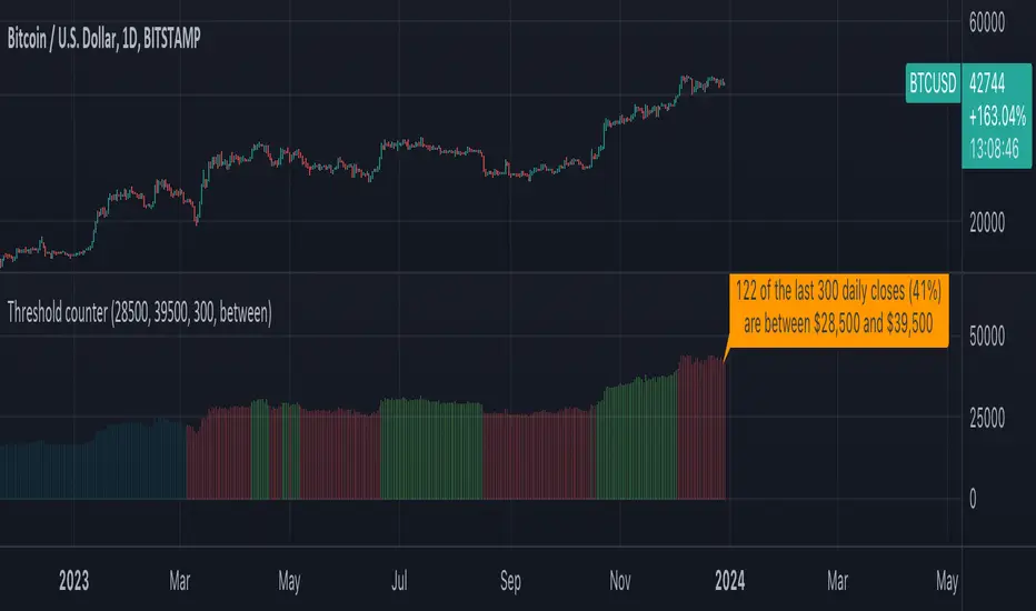
🔥 SMC Reversal Engine v3.5 – Clean FVG + DashboardSMC Reversal Engine v3.5 – Clean FVG + Dashboard
The SMC Reversal Engine is a precision-built Smart Money Concepts tool designed to help traders understand market structure the single most important foundation in reading price action. It reveals how institutions move liquidity, where structure shifts occur, and how Fair Value Gaps (FVGs) align with these changes to signal potential reversals or continuations.
Understanding How It Works
At its core, the script detects CHoCH (Change of Character) and BOS (Break of Structure)—the two key turning points in institutional order flow. A CHoCH shows that the market has reversed intent (for example, from bearish to bullish), while a BOS confirms a continuation of the current trend. Together, they form the backbone of structure-based trading.
To refine this logic, the engine uses fractal pivots clusters of candles that confirm swing highs and lows. Fractals filter out noise, identifying points where price truly changes direction. The script lets you set this sensitivity manually or automatically adapts it depending on the timeframe. Lower fractal sensitivity captures smaller intraday swings for scalpers, while higher sensitivity locks onto major swing structures for swing and position traders.
The dashboard gives you a real-time reading of the trend, the last high and low, and what the market is likely to do next—for example, “Expect HL” or “Wait for LH.” It even tracks the accuracy of these structure predictions over time, giving an educational feedback loop to help you learn price behavior.
Fair Value Gaps and Tap Entries
Fair Value Gaps (FVGs) mark moments when price moves too quickly, leaving inefficiencies that institutions often revisit. When price taps into an FVG, it often acts as a high-probability entry zone for reversals or continuations. The script automatically detects, extends, and deletes old FVGs, keeping only relevant zones visible for a clean chart.
Traders can enable markTapEntry to visually confirm when an FVG gets filled. This is a simple but powerful trigger that often aligns with CHoCH or BOS moments.
Recommended Settings for Different Traders
For Scalpers, use a lower HTF structure such as 1 minute or 5 minutes. Keep Auto Fractals on for faster reaction, and limit FVG zones to 2–3. This gives you a clean, real-time reflection of order flow.
For Intraday Traders, 15-minute to 1-hour structure gives the perfect balance between reactivity and stability. Fractal sensitivity around 3–5 captures the most actionable levels without excessive noise.
For Swing Traders, use 4-hour, 1-day, or even 3-day structure. The chart becomes smoother, showing higher-order CHoCH and BOS that define true institutional transitions. Combine this with EMA confirmation for higher conviction.
For Position or Macro Traders, select Weekly or Monthly structure. The dynamic label system expands automatically to keep more historical BOS/CHoCH points visible, allowing you to see long-term shifts clearly.
Educational Value
This indicator is built to teach traders how to see structure the way professionals and smart money do. You’ll learn to recognize how markets transition from one phase to another from accumulation to manipulation to expansion. Each CHoCH or BOS helps you decode where liquidity is being taken and where new intent begins.
The included SMC Quick Guide explains each structural cue right on your chart. Within days of using it, you’ll start noticing patterns that reveal how price really moves, instead of guessing based on indicators.
Settings and How to Use Them
Everything in the SMC Reversal Engine is designed to adapt to your trading style and help you read structure like a professional.
When you open the Inputs Panel, you’ll see sections like Fractal Settings, FVG Settings, Buy/Sell Confirmation, and Educational Tools.
Under Fractal Settings, you can choose the higher timeframe (HTF) that defines structure—from minutes to weeks. The Auto Fractal Sensitivity option automatically adjusts how tight or wide swing points are detected. Lower sensitivity captures short-term fluctuations (great for scalpers), while higher values filter noise and isolate major swing highs and lows (perfect for swing traders).
The Fair Value Gap (FVG) options manage imbalance zones—the footprints of institutional orders. You can show or hide these zones, extend them into the future, and control how long they remain before auto-deletion. The Mark Entry When FVG is Tapped option places a small label when price revisits the gap—a potential entry signal that aligns with smart money logic.
EMA Confirmation adds a layer of confluence. The script can automatically scale EMA lengths based on timeframe, or you can input your preferred values (for example, 9/21 for intraday, 50/200 for swing). Require EMA Crossover Confirmation helps filter false moves, keeping you trading only with aligned momentum.
The Educational section gives traders visual reinforcement. When enabled, you’ll see tags like HH (Higher High), HL (Higher Low), LH (Lower High), and LL (Lower Low). These show structure shifts in real time, helping you learn visually what market structure really means. The Cheat Sheet panel summarizes each term, always visible in the corner for quick reference.
Early Top Warnings use wick size and RSI divergence to signal when price may be overextended—a useful heads-up before potential CHoCH formations.
Finally, the Narrative and Accuracy System translates structure into simple English—messages like Trend Bullish → Wait for HL or BOS Bearish → Expect LL. Over time, you can monitor how accurate these expectations have been, training your pattern recognition and confidence.
Pro Tips for Getting the Most Out of the SMC Reversal Engine
1. Start on Higher Timeframes First: Begin on the 4H or Daily chart where structure is cleaner and signals have more weight. Then scale down for entries once you grasp directional intent.
2. Use FVGs for Context, Not Just Entries: Observe how price behaves around unfilled FVGs—they often act as magnets or barriers, offering insight into where liquidity lies.
3. Combine With HTF Bias: Always trade in the direction of your higher timeframe trend. A bullish weekly BOS means lower timeframes should ideally align bullishly for optimal setups.
4. Clean Charts = Clear Mind: Use Minimal Mode when focusing on price action, then toggle the educational tools back on to review structure for learning.
5. Don’t Chase Every CHoCH or BOS: Focus on significant breaks that align with broader context and liquidity sweeps, not minor fluctuations.
6. Accuracy Rate Is a Feedback Tool: Use the accuracy stat as a reflection of consistency—not a trade trigger.
7. Build Narrative Awareness: Read the on-chart narrative messages to reinforce structured thinking and stay disciplined.
8. Practice Replay Mode: Step through past structures to visually connect CHoCH, BOS, and FVG behavior. It’s one of the best ways to train pattern recognition.
Summary
* Detects CHoCH and BOS automatically with fractal precision
* Identifies and manages Fair Value Gaps (FVGs) in real time
* Displays a smart dashboard with accuracy tracking
* Adapts label visibility dynamically by timeframe
* Perfect for both learning and trading with institutional clarity
This tool isn’t about predicting the market—it’s about understanding it. Once you can read structure, everything else in trading becomes secondary.
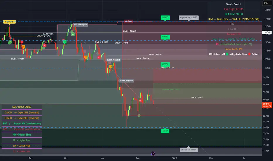
Volumatic VIDYA – Pro+1. Professional & Clear (recommended for TradingView)
Volumatic VIDYA Pro+ combines a dynamic VIDYA trend filter, Delta Volume pressure, and automatic pattern recognition (Double/Triple Tops & Bottoms, Head & Shoulders).
A complete technical tool for detecting momentum shifts, trend reversals, and trade entries across multiple timeframes.
2. Short & Catchy
Adaptive VIDYA trendline + Delta Volume + Pattern detection in one tool.
Instantly visualize market bias, structure, and momentum strength.
3. Educational / Analytical
Analyze market dynamics with VIDYA-based trend filtering, volume delta analysis, and automated pattern recognition.
Ideal for traders who combine price action with quantitative confirmation.

Mean Reversion Oscillator [Alpha Extract]An advanced composite oscillator system specifically designed to identify extreme market conditions and high-probability mean reversion opportunities, combining five proven oscillators into a single, powerful analytical framework.
By integrating multiple momentum and volume-based indicators with sophisticated extreme level detection, this oscillator provides precise entry signals for contrarian trading strategies while filtering out false reversals through momentum confirmation.
🔶 Multi-Oscillator Composite Framework
Utilizes a comprehensive approach that combines Bollinger %B, RSI, Stochastic, Money Flow Index, and Williams %R into a unified composite score. This multi-dimensional analysis ensures robust signal generation by capturing different aspects of market extremes and momentum shifts.
// Weighted composite (equal weights)
normalized_bb = bb_percent
normalized_rsi = rsi
normalized_stoch = stoch_d_val
normalized_mfi = mfi
normalized_williams = williams_r
composite_raw = (normalized_bb + normalized_rsi + normalized_stoch + normalized_mfi + normalized_williams) / 5
composite = ta.sma(composite_raw, composite_smooth)
🔶 Advanced Extreme Level Detection
Features a sophisticated dual-threshold system that distinguishes between moderate and extreme market conditions. This hierarchical approach allows traders to identify varying degrees of mean reversion potential, from moderate oversold/overbought conditions to extreme levels that demand immediate attention.
🔶 Momentum Confirmation System
Incorporates a specialized momentum histogram that confirms mean reversion signals by analyzing the rate of change in the composite oscillator. This prevents premature entries during strong trending conditions while highlighting genuine reversal opportunities.
// Oscillator momentum (rate of change)
osc_momentum = ta.mom(composite, 5)
histogram = osc_momentum
// Momentum confirmation
momentum_bullish = histogram > histogram
momentum_bearish = histogram < histogram
// Confirmed signals
confirmed_bullish = bullish_entry and momentum_bullish
confirmed_bearish = bearish_entry and momentum_bearish
🔶 Dynamic Visual Intelligence
The oscillator line adapts its color intensity based on proximity to extreme levels, providing instant visual feedback about market conditions. Background shading creates clear zones that highlight when markets enter moderate or extreme territories.
🔶 Intelligent Signal Generation
Generates precise entry signals only when the composite oscillator crosses extreme thresholds with momentum confirmation. This dual-confirmation approach significantly reduces false signals while maintaining sensitivity to genuine mean reversion opportunities.
How It Works
🔶 Composite Score Calculation
The indicator simultaneously tracks five different oscillators, each normalized to a 0-100 scale, then combines them into a smoothed composite score. This approach eliminates the noise inherent in single-oscillator analysis while capturing the consensus view of multiple momentum indicators.
// Mean reversion entry signals
bullish_entry = ta.crossover(composite, 100 - extreme_level) and composite < (100 - extreme_level)
bearish_entry = ta.crossunder(composite, extreme_level) and composite > extreme_level
// Bollinger %B calculation
bb_basis = ta.sma(src, bb_length)
bb_dev = bb_mult * ta.stdev(src, bb_length)
bb_percent = (src - bb_lower) / (bb_upper - bb_lower) * 100
🔶 Extreme Zone Identification
The system automatically identifies when markets reach statistically significant extreme levels, both moderate (65/35) and extreme (80/20). These zones represent areas where mean reversion has the highest probability of success based on historical market behavior.
🔶 Momentum Histogram Analysis
A specialized momentum histogram tracks the velocity of oscillator changes, helping traders distinguish between healthy corrections and potential trend reversals. The histogram's color-coded display makes momentum shifts immediately apparent.
🔶 Divergence Detection Framework
Built-in divergence analysis identifies situations where price and oscillator movements diverge, often signaling impending reversals. Diamond-shaped markers highlight these critical divergence patterns for enhanced pattern recognition.
🔶 Real-Time Information Dashboard
An integrated information table provides instant access to current oscillator readings, market status, and individual component values. This dashboard eliminates the need to manually check multiple indicators while trading.
🔶 Individual Component Display
Optional display of individual oscillator components allows traders to understand which specific indicators are driving the composite signal. This transparency enables more informed decision-making and deeper market analysis.
🔶 Adaptive Background Coloring
Intelligent background shading automatically adjusts based on market conditions, creating visual zones that correspond to different levels of mean reversion potential. The subtle color gradations make pattern recognition effortless.
1D
3D
🔶 Comprehensive Alert System
Multi-tier alert system covers confirmed entry signals, divergence patterns, and extreme level breaches. Each alert type provides specific context about the detected condition, enabling traders to respond appropriately to different signal strengths.
🔶 Customizable Threshold Management
Fully adjustable extreme and moderate levels allow traders to fine-tune the indicator's sensitivity to match different market volatilities and trading timeframes. This flexibility ensures optimal performance across various market conditions.
🔶 Why Choose AE - Mean Reversion Oscillator?
This indicator provides the most comprehensive approach to mean reversion trading by combining multiple proven oscillators with advanced confirmation mechanisms. By offering clear visual hierarchies for different extreme levels and requiring momentum confirmation for signals, it empowers traders to identify high-probability contrarian opportunities while avoiding false reversals. The sophisticated composite methodology ensures that signals are both statistically significant and practically actionable, making it an essential tool for traders focused on mean reversion strategies across all market conditions.